Spark vs Hadoop 1 Spark Set of concise

Spark vs Hadoop 1

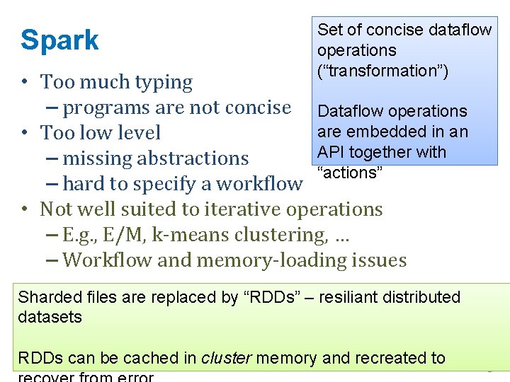
Spark Set of concise dataflow operations (“transformation”) • Too much typing – programs are not concise Dataflow operations are embedded in an • Too low level API together with – missing abstractions “actions” – hard to specify a workflow • Not well suited to iterative operations – E. g. , E/M, k-means clustering, … – Workflow and memory-loading issues Sharded files are replaced by “RDDs” – resiliant distributed datasets RDDs can be cached in cluster memory and recreated to 2

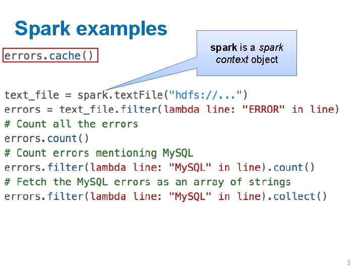
Spark examples spark is a spark context object 3

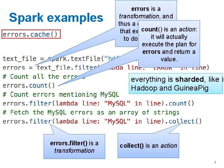
Spark examples errors is a transformation, and thus a data strucure count() is an action: that explains HOW it will actually to do something execute the plan for errors and return a value. everything is sharded, like in Hadoop and Guinea. Pig errors. filter() is a transformation collect() is an action 4

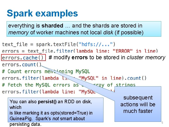
Spark examples everything is sharded … and the shards are stored in memory of worker machines not local disk (if possible) # modify errors to be stored in cluster memory You can also persist() an RDD on disk, which is like marking it as opts(stored=True) in Guinea. Pig. Spark’s not smart about persisting data. subsequent actions will be much faster 5

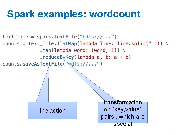
Spark examples: wordcount the action transformation on (key, value) pairs , which are special 6

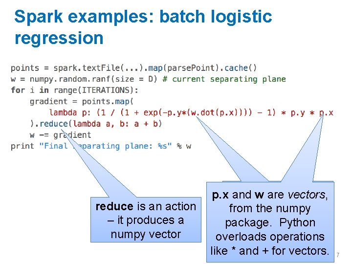
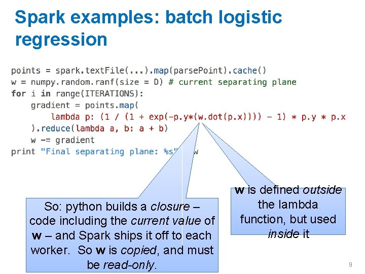
Spark examples: batch logistic regression reduce is an action – it produces a numpy vector p. xwand are p. x and are w vectors, from the numpy package. Python overloads operations like * and + for vectors. 7

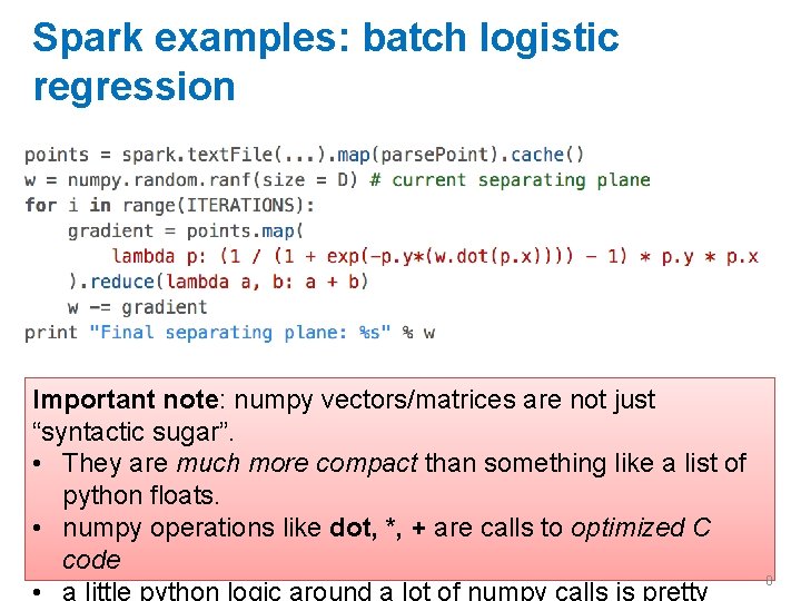
Spark examples: batch logistic regression Important note: numpy vectors/matrices are not just “syntactic sugar”. • They are much more compact than something like a list of python floats. • numpy operations like dot, *, + are calls to optimized C code • a little python logic around a lot of numpy calls is pretty 8

Spark examples: batch logistic regression So: python builds a closure – code including the current value of w – and Spark ships it off to each worker. So w is copied, and must be read-only. w is defined outside the lambda function, but used inside it 9

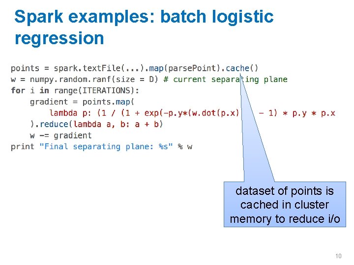
Spark examples: batch logistic regression dataset of points is cached in cluster memory to reduce i/o 10

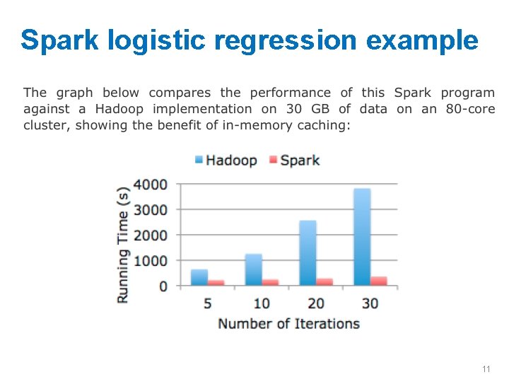
Spark logistic regression example 11

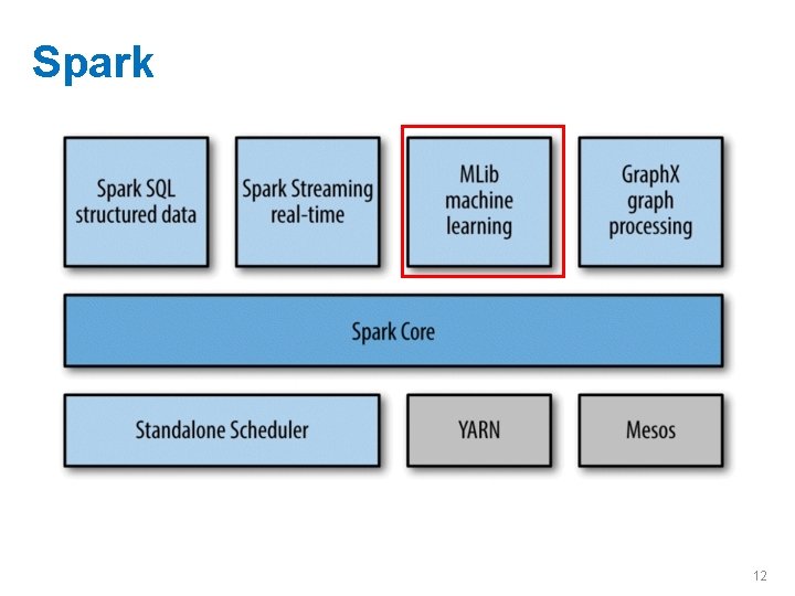
Spark 12

Other Map-Reduce (ish) Frameworks William Cohen 17

MAP-REDUCE ABSTRACTIONS: CASCADING, PIPES, SCALDING 18

Y: Y=Hadoop+X • Cascading – Java library for map-reduce workflows – Also some library operations for common mappers/reducers 19

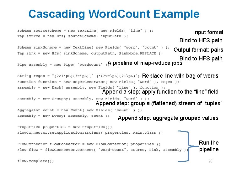
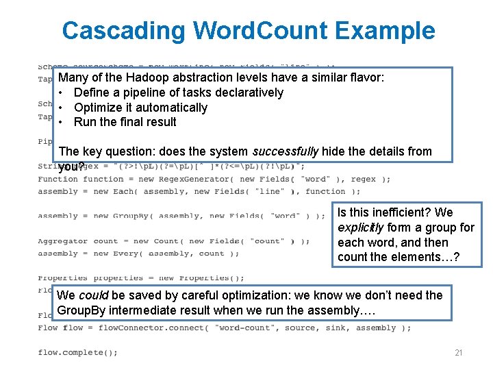
Cascading Word. Count Example Input format Bind to HFS path Output format: pairs Bind to HFS path A pipeline of map-reduce jobs Replace line with bag of words Append a step: apply function to the “line” field Append step: group a (flattened) stream of “tuples” Append step: aggregate grouped values Run the pipeline 20

Cascading Word. Count Example Many of the Hadoop abstraction levels have a similar flavor: • Define a pipeline of tasks declaratively • Optimize it automatically • Run the final result The key question: does the system successfully hide the details from you? Is this inefficient? We explicitly form a group for each word, and then count the elements…? We could be saved by careful optimization: we know we don’t need the Group. By intermediate result when we run the assembly…. 21

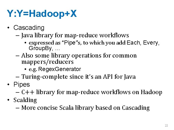
Y: Y=Hadoop+X • Cascading – Java library for map-reduce workflows • expressed as “Pipe”s, to which you add Each, Every, Group. By, … – Also some library operations for common mappers/reducers • e. g. Regex. Generator – Turing-complete since it’s an API for Java • Pipes – C++ library for map-reduce workflows on Hadoop • Scalding – More concise Scala library based on Cascading 22

MORE DECLARATIVE LANGUAGES 23

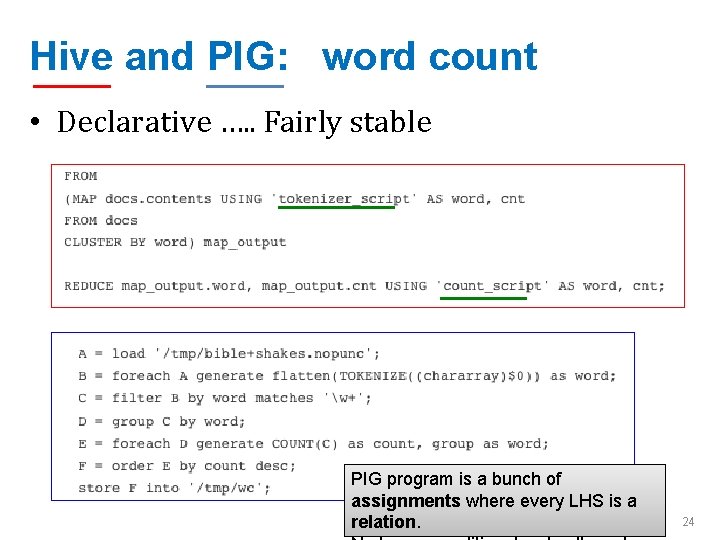
Hive and PIG: word count • Declarative …. . Fairly stable PIG program is a bunch of assignments where every LHS is a relation. 24

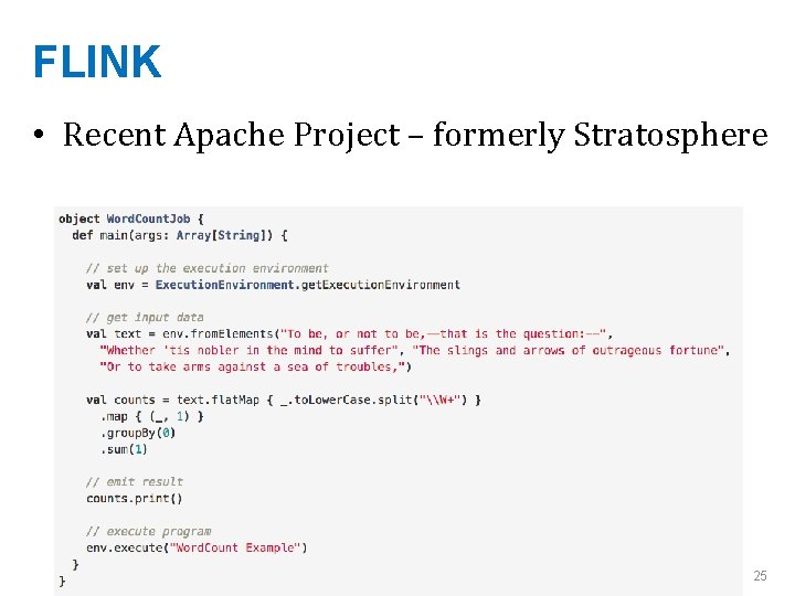
FLINK • Recent Apache Project – formerly Stratosphere …. 25

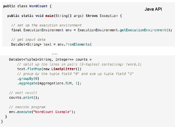
Java API FLINK • Apache Project – just getting started …. 26

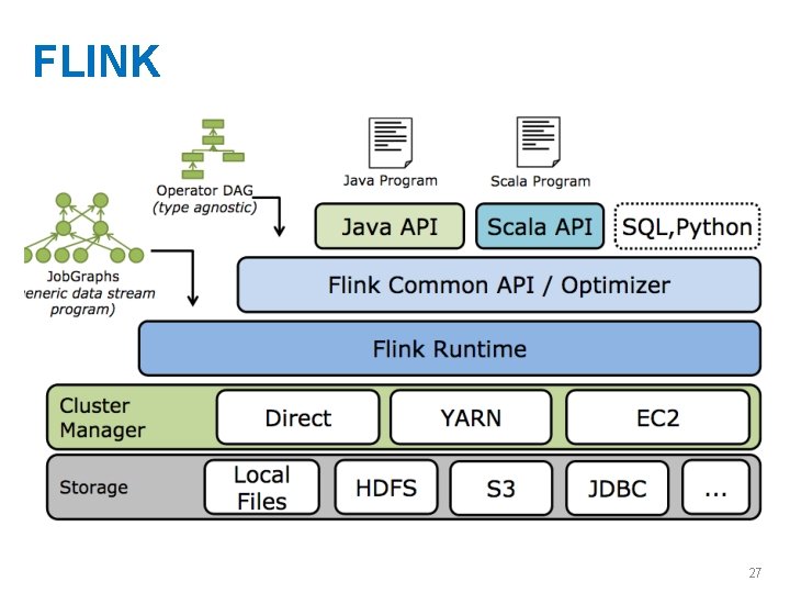
FLINK 27

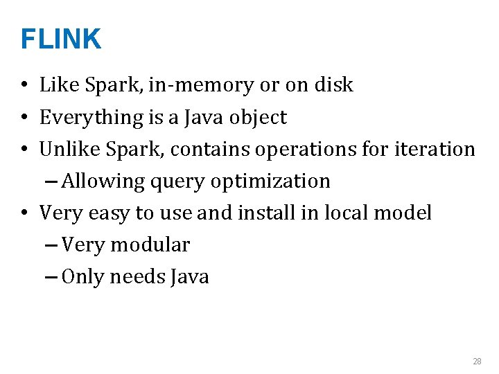
FLINK • Like Spark, in-memory or on disk • Everything is a Java object • Unlike Spark, contains operations for iteration – Allowing query optimization • Very easy to use and install in local model – Very modular – Only needs Java 28

One more algorithm to discuss as a Map-reduce implementation…. 29

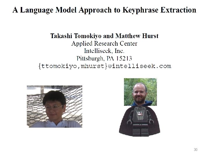
30

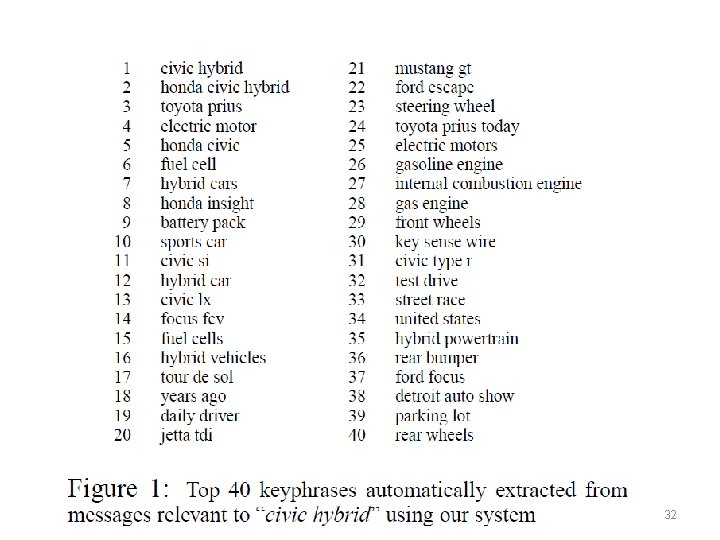
32

Why phrase-finding? • There are lots of phrases • There’s not supervised data • It’s hard to articulate – What makes a phrase, vs just an ngram? • a phrase is independently meaningful (“test drive”, “red meat”) or not (“are interesting”, “are lots”) – What makes a phrase interesting? 33

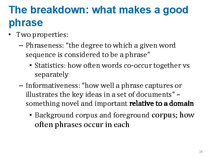
The breakdown: what makes a good phrase • Two properties: – Phraseness: “the degree to which a given word sequence is considered to be a phrase” • Statistics: how often words co-occur together vs separately – Informativeness: “how well a phrase captures or illustrates the key ideas in a set of documents” – something novel and important relative to a domain • Background corpus and foreground corpus; how often phrases occur in each 34

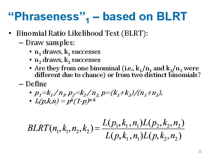
“Phraseness” 1 – based on BLRT • Binomial Ratio Likelihood Test (BLRT): – Draw samples: • n 1 draws, k 1 successes • n 2 draws, k 2 successes • Are they from one binominal (i. e. , k 1/n 1 and k 2/n 2 were different due to chance) or from two distinct binomials? – Define • p 1=k 1 / n 1, p 2=k 2 / n 2, p=(k 1+k 2)/(n 1+n 2), • L(p, k, n) = pk(1 -p)n-k 35

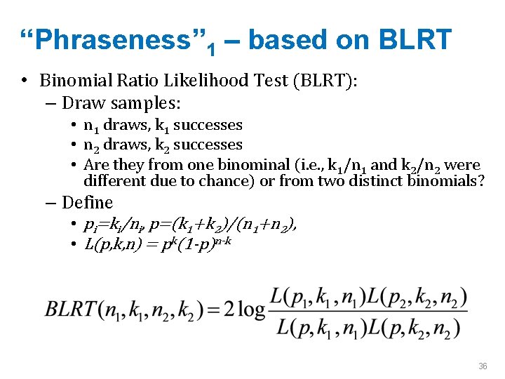
“Phraseness” 1 – based on BLRT • Binomial Ratio Likelihood Test (BLRT): – Draw samples: • n 1 draws, k 1 successes • n 2 draws, k 2 successes • Are they from one binominal (i. e. , k 1/n 1 and k 2/n 2 were different due to chance) or from two distinct binomials? – Define • pi=ki/ni, p=(k 1+k 2)/(n 1+n 2), • L(p, k, n) = pk(1 -p)n-k 36

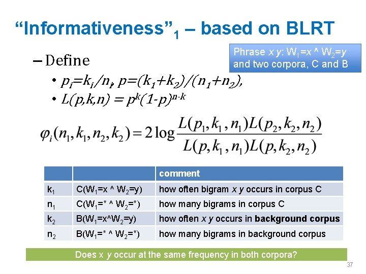
“Informativeness” 1 – based on BLRT Phrase x y: W 1=x ^ W 2=y and two corpora, C and B – Define • pi=ki /ni, p=(k 1+k 2)/(n 1+n 2), • L(p, k, n) = pk(1 -p)n-k comment k 1 C(W 1=x ^ W 2=y) how often bigram x y occurs in corpus C n 1 C(W 1=* ^ W 2=*) how many bigrams in corpus C k 2 B(W 1=x^W 2=y) how often x y occurs in background corpus n 2 B(W 1=* ^ W 2=*) how many bigrams in background corpus Does x y occur at the same frequency in both corpora? 37

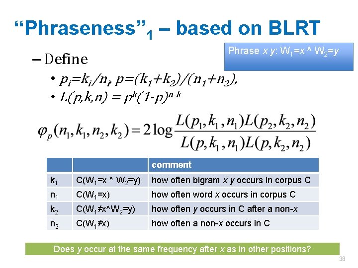
“Phraseness” 1 – based on BLRT Phrase x y: W 1=x ^ W 2=y – Define • pi=ki /ni, p=(k 1+k 2)/(n 1+n 2), • L(p, k, n) = pk(1 -p)n-k comment k 1 C(W 1=x ^ W 2=y) how often bigram x y occurs in corpus C n 1 C(W 1=x) how often word x occurs in corpus C k 2 C(W 1≠x^W 2=y) how often y occurs in C after a non-x n 2 C(W 1≠x) how often a non-x occurs in C Does y occur at the same frequency after x as in other positions? 38

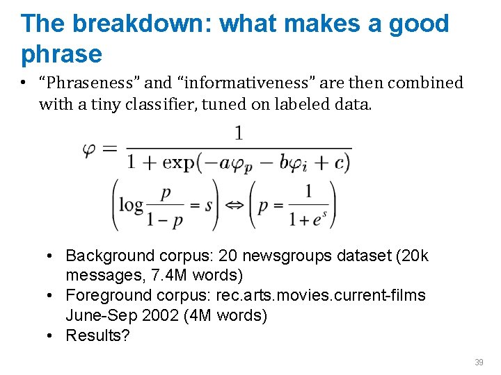
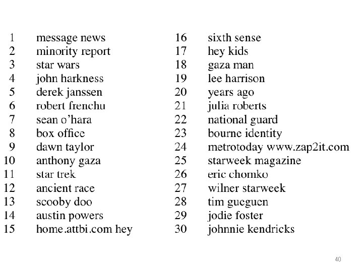
The breakdown: what makes a good phrase • “Phraseness” and “informativeness” are then combined with a tiny classifier, tuned on labeled data. • Background corpus: 20 newsgroups dataset (20 k messages, 7. 4 M words) • Foreground corpus: rec. arts. movies. current-films June-Sep 2002 (4 M words) • Results? 39

40

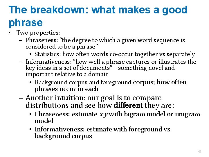
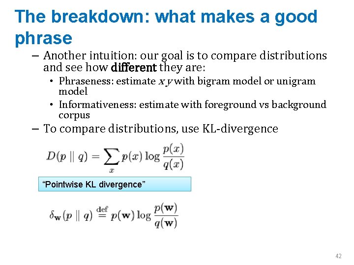
The breakdown: what makes a good phrase • Two properties: – Phraseness: “the degree to which a given word sequence is considered to be a phrase” • Statistics: how often words co-occur together vs separately – Informativeness: “how well a phrase captures or illustrates the key ideas in a set of documents” – something novel and important relative to a domain • Background corpus and foreground corpus; how often phrases occur in each – Another intuition: our goal is to compare distributions and see how different they are: • Phraseness: estimate x y with bigram model or unigram model • Informativeness: estimate with foreground vs background corpus 41

The breakdown: what makes a good phrase – Another intuition: our goal is to compare distributions and see how different they are: • Phraseness: estimate x y with bigram model or unigram model • Informativeness: estimate with foreground vs background corpus – To compare distributions, use KL-divergence “Pointwise KL divergence” 42

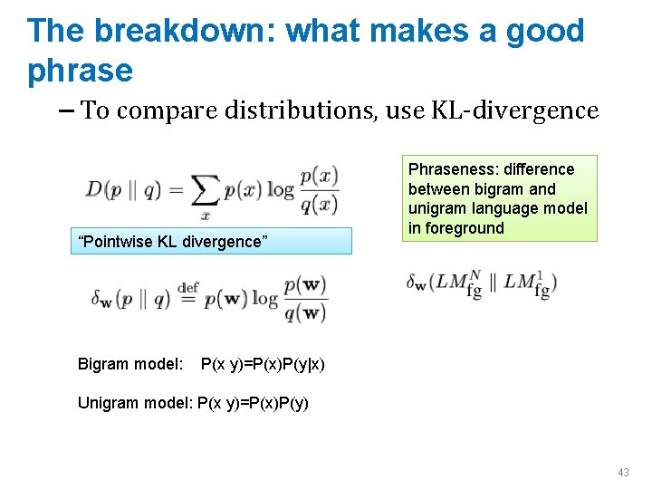
The breakdown: what makes a good phrase – To compare distributions, use KL-divergence “Pointwise KL divergence” Bigram model: Phraseness: difference between bigram and unigram language model in foreground P(x y)=P(x)P(y|x) Unigram model: P(x y)=P(x)P(y) 43

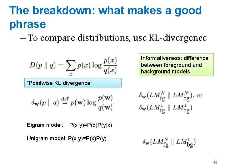
The breakdown: what makes a good phrase – To compare distributions, use KL-divergence Informativeness: difference between foreground and background models “Pointwise KL divergence” Bigram model: P(x y)=P(x)P(y|x) Unigram model: P(x y)=P(x)P(y) 44

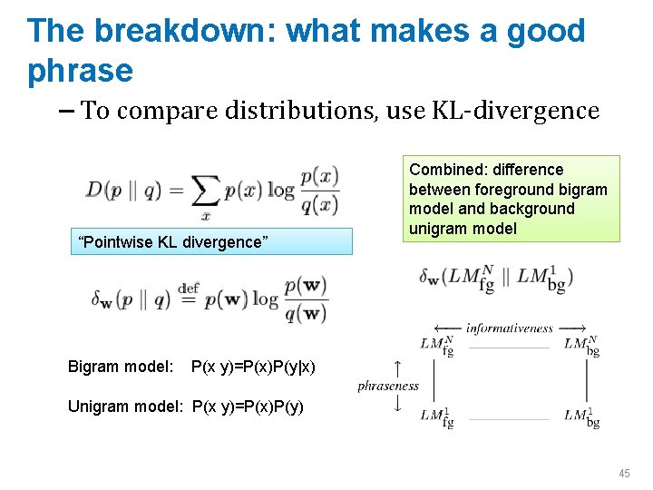
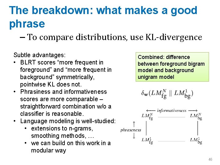
The breakdown: what makes a good phrase – To compare distributions, use KL-divergence “Pointwise KL divergence” Bigram model: Combined: difference between foreground bigram model and background unigram model P(x y)=P(x)P(y|x) Unigram model: P(x y)=P(x)P(y) 45

The breakdown: what makes a good phrase – To compare distributions, use KL-divergence Subtle advantages: • BLRT scores “more frequent in foreground” and “more frequent in background” symmetrically, pointwise KL does not. • Phrasiness and informativeness scores are more comparable – straightforward combination w/o a classifier is reasonable. • Language modeling is well-studied: • extensions to n-grams, smoothing methods, … • we can build on this work in a modular way Combined: difference between foreground bigram model and background unigram model 46

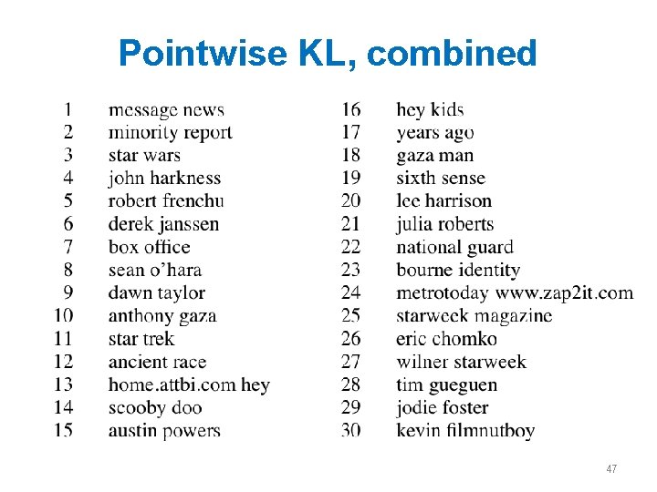
Pointwise KL, combined 47

Why phrase-finding? • Phrases are where the standard supervised “bag of words” representation starts to break. • There’s not supervised data, so it’s hard to see what’s “right” and why • It’s a nice example of using unsupervised signals to solve a task that could be formulated as supervised learning • It’s a nice level of complexity, if you want to do it in a scalable way. 48

Phrase Finding in Guinea Pig 49

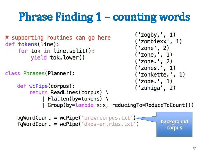
Phrase Finding 1 – counting words background corpus 50

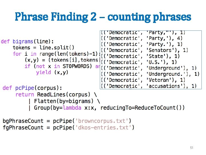
Phrase Finding 2 – counting phrases 51

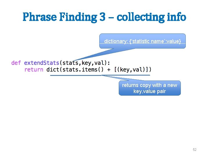
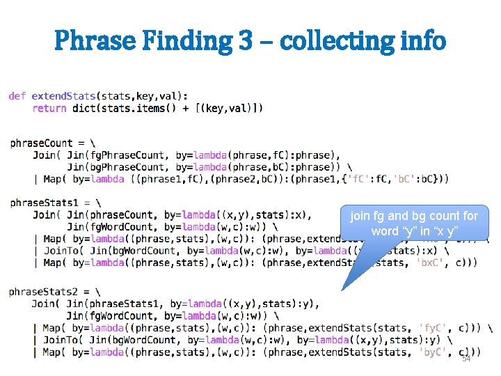
Phrase Finding 3 – collecting info dictionary: {‘statistic name’: value} returns copy with a new key, value pair 52

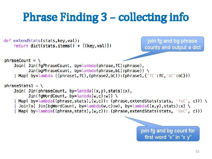
Phrase Finding 3 – collecting info join fg and bg phrase counts and output a dict join fg and bg count for first word “x” in “x y” 53

Phrase Finding 3 – collecting info join fg and bg count for word “y” in “x y” 54

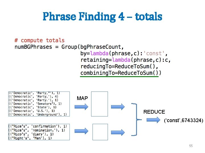
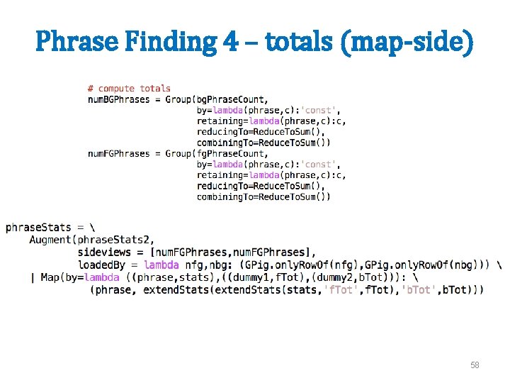
Phrase Finding 4 – totals MAP REDUCE (‘const’, 6743324) 55

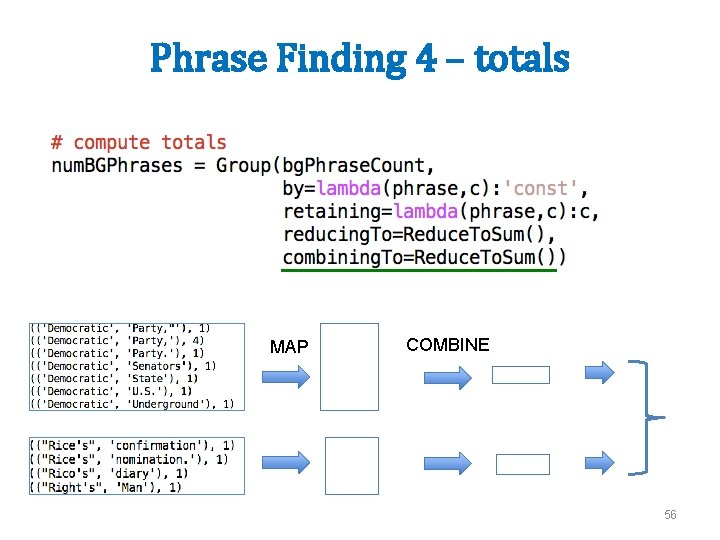
Phrase Finding 4 – totals MAP COMBINE 56

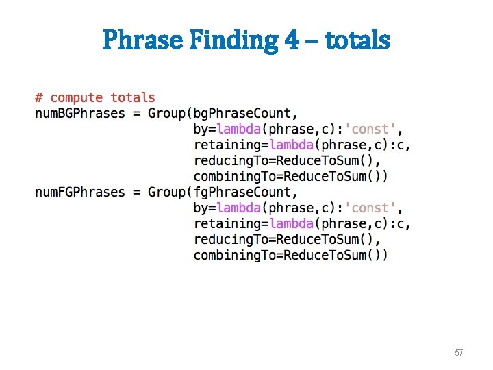
Phrase Finding 4 – totals 57

Phrase Finding 4 – totals (map-side) 58

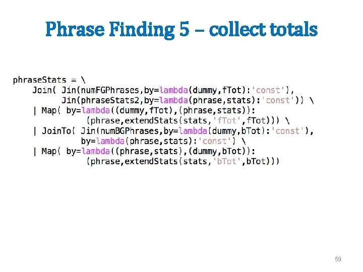
Phrase Finding 5 – collect totals 59

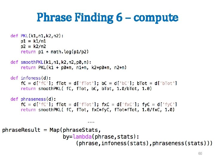
Phrase Finding 6 – compute …. 60

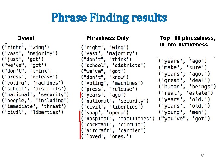
Phrase Finding results Overall Phrasiness Only Top 100 phraseiness, lo informativeness 61

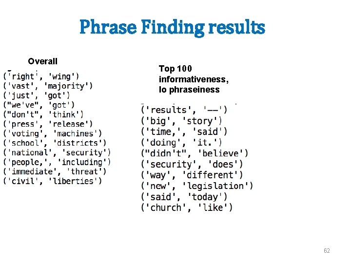
Phrase Finding results Overall Top 100 informativeness, lo phraseiness 62

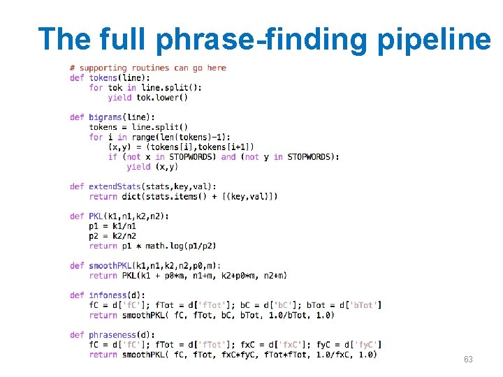
The full phrase-finding pipeline 63

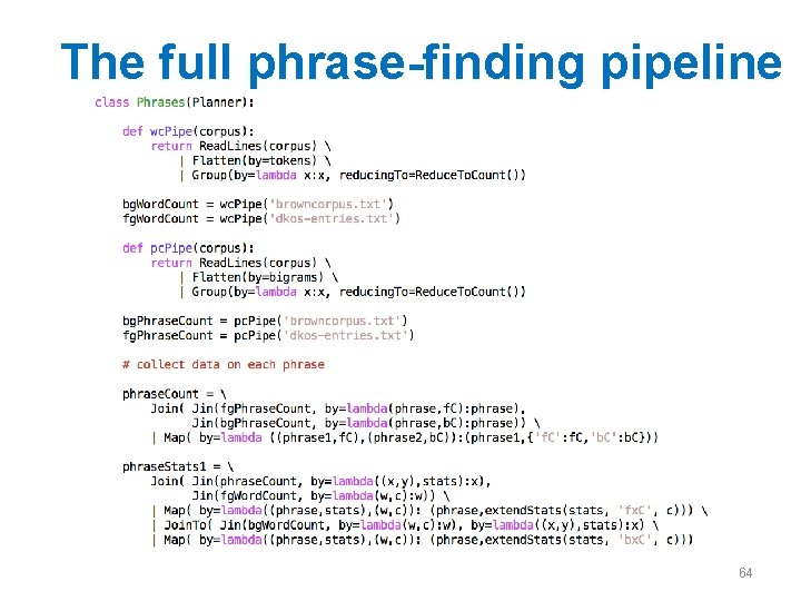
The full phrase-finding pipeline 64

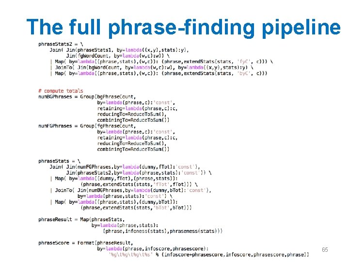
The full phrase-finding pipeline 65

Phrase Finding in PIG 66

Phrase Finding 1 - loading the input 67

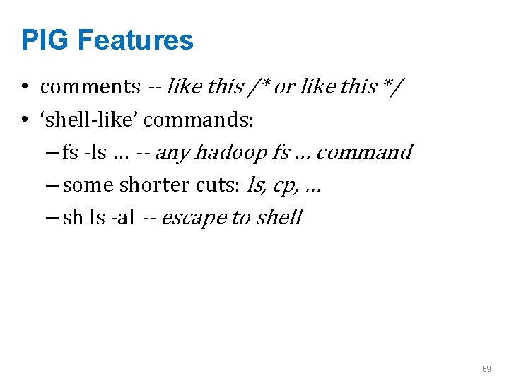
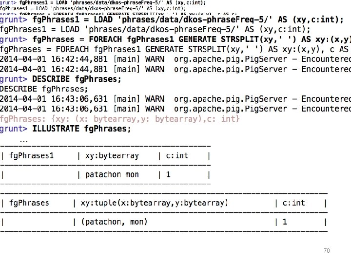
PIG Features • comments -- like this /* or like this */ • ‘shell-like’ commands: – fs -ls … -- any hadoop fs … command – some shorter cuts: ls, cp, … – sh ls -al -- escape to shell 69

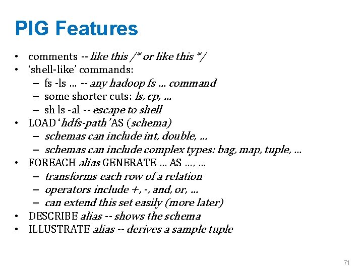
PIG Features • comments -- like this /* or like this */ • ‘shell-like’ commands: – fs -ls … -- any hadoop fs … command – some shorter cuts: ls, cp, … – sh ls -al -- escape to shell • LOAD ‘hdfs-path’ AS (schema) – schemas can include int, double, … – schemas can include complex types: bag, map, tuple, … • FOREACH alias GENERATE … AS …, … – transforms each row of a relation – operators include +, -, and, or, … – can extend this set easily (more later) • DESCRIBE alias -- shows the schema • ILLUSTRATE alias -- derives a sample tuple 71

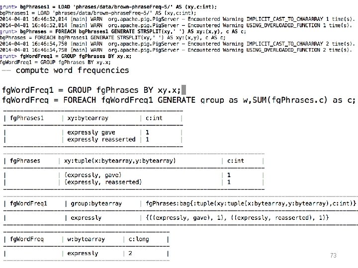
Phrase Finding 1 - word counts 72

73

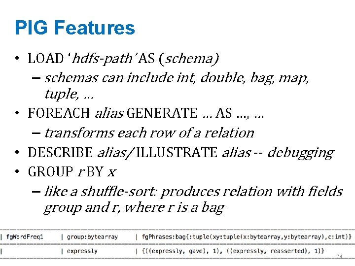
PIG Features • LOAD ‘hdfs-path’ AS (schema) – schemas can include int, double, bag, map, tuple, … • FOREACH alias GENERATE … AS …, … – transforms each row of a relation • DESCRIBE alias/ ILLUSTRATE alias -- debugging • GROUP r BY x – like a shuffle-sort: produces relation with fields group and r, where r is a bag 74

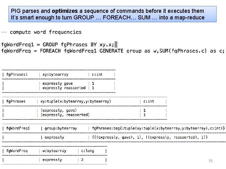
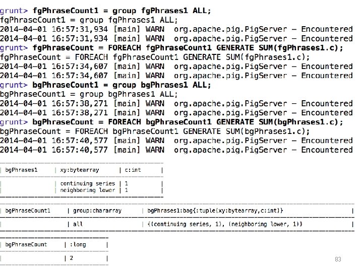
PIG parses and optimizes a sequence of commands before it executes them It’s smart enough to turn GROUP … FOREACH… SUM … into a map-reduce 75

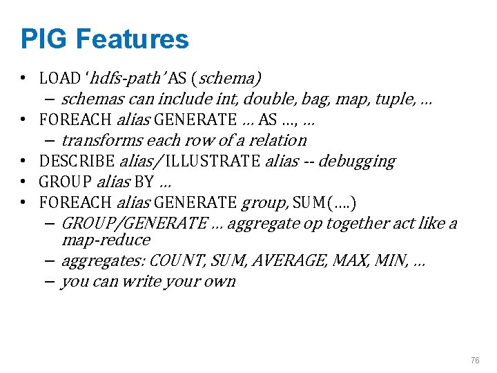
PIG Features • LOAD ‘hdfs-path’ AS (schema) – schemas can include int, double, bag, map, tuple, … • FOREACH alias GENERATE … AS …, … – transforms each row of a relation • DESCRIBE alias/ ILLUSTRATE alias -- debugging • GROUP alias BY … • FOREACH alias GENERATE group, SUM(…. ) – GROUP/GENERATE … aggregate op together act like a map-reduce – aggregates: COUNT, SUM, AVERAGE, MAX, MIN, … – you can write your own 76

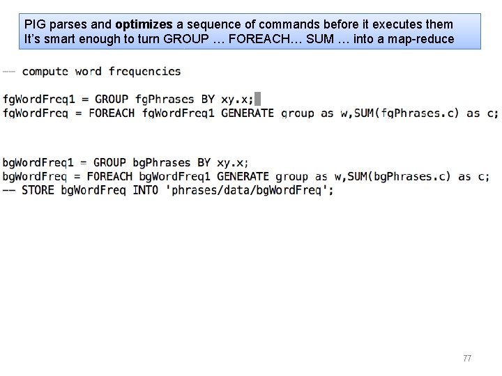
PIG parses and optimizes a sequence of commands before it executes them It’s smart enough to turn GROUP … FOREACH… SUM … into a map-reduce 77

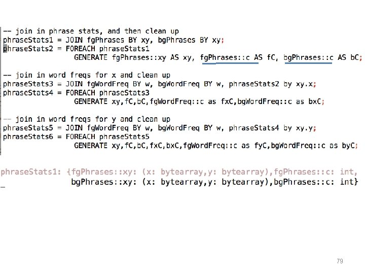
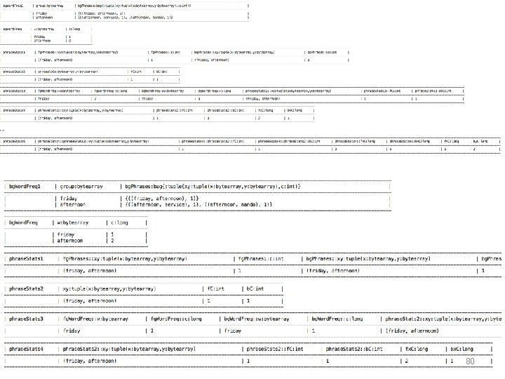
Phrase Finding 3 - assembling phrase- and word-level statistics 78

79

80

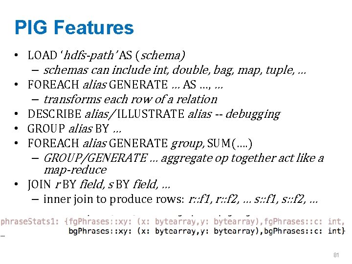
PIG Features • LOAD ‘hdfs-path’ AS (schema) – schemas can include int, double, bag, map, tuple, … • FOREACH alias GENERATE … AS …, … – transforms each row of a relation • DESCRIBE alias/ ILLUSTRATE alias -- debugging • GROUP alias BY … • FOREACH alias GENERATE group, SUM(…. ) – GROUP/GENERATE … aggregate op together act like a map-reduce • JOIN r BY field, s BY field, … – inner join to produce rows: r: : f 1, r: : f 2, … s: : f 1, s: : f 2, … 81

Phrase Finding 4 - adding total frequencies 82

83

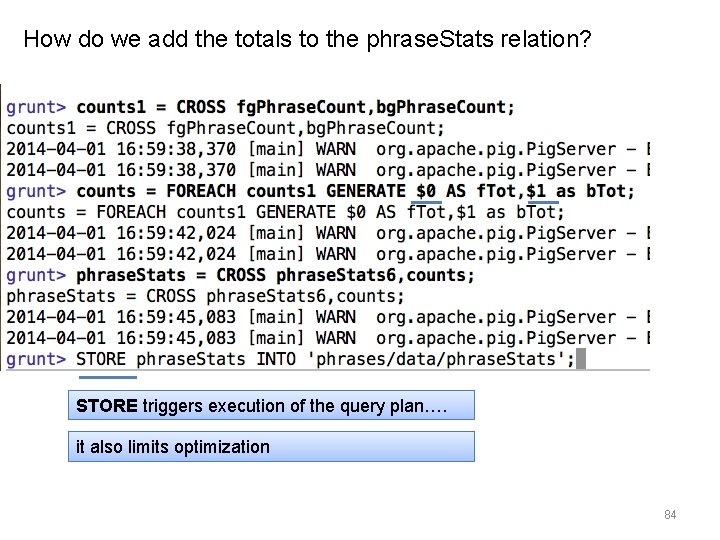
How do we add the totals to the phrase. Stats relation? STORE triggers execution of the query plan…. it also limits optimization 84

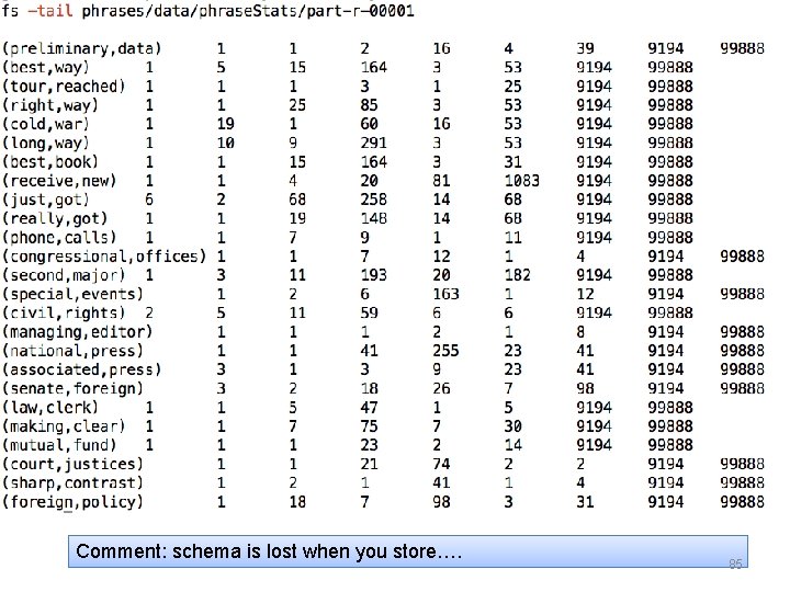
Comment: schema is lost when you store…. 85

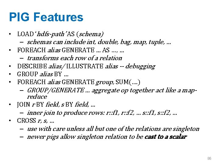
PIG Features • LOAD ‘hdfs-path’ AS (schema) – schemas can include int, double, bag, map, tuple, … • FOREACH alias GENERATE … AS …, … – transforms each row of a relation • DESCRIBE alias/ ILLUSTRATE alias -- debugging • GROUP alias BY … • FOREACH alias GENERATE group, SUM(…. ) – GROUP/GENERATE … aggregate op together act like a mapreduce • JOIN r BY field, s BY field, … – inner join to produce rows: r: : f 1, r: : f 2, … s: : f 1, s: : f 2, … • CROSS r, s, … – use with care unless all but one of the relations are singleton – newer pigs allow singleton relation to be cast to a scalar 86

Phrase Finding 5 - phrasiness and informativeness 87

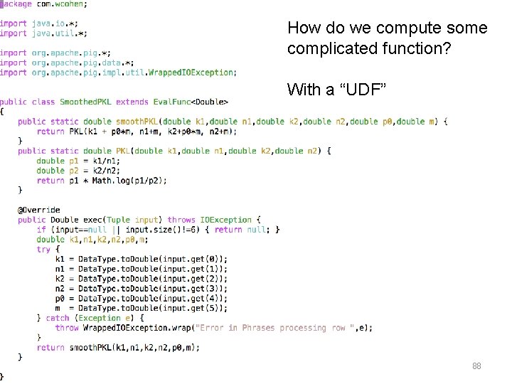
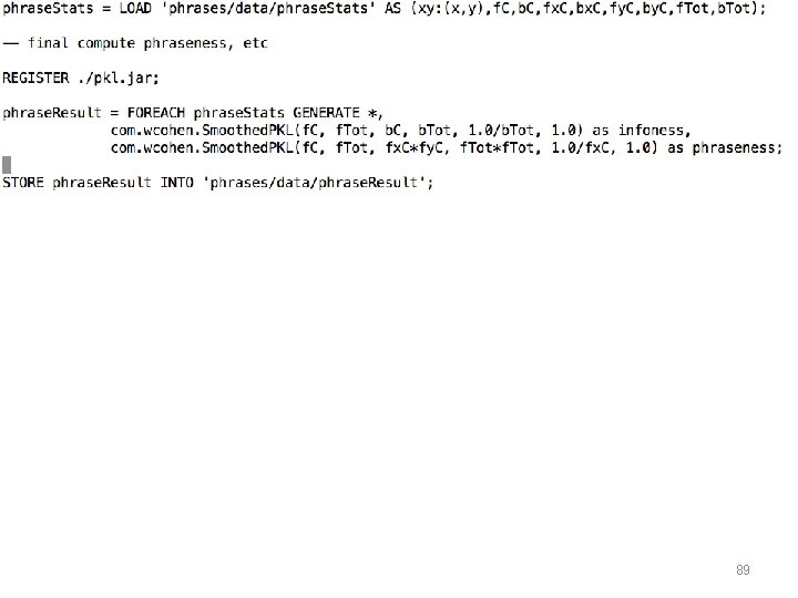
How do we compute some complicated function? With a “UDF” 88

89

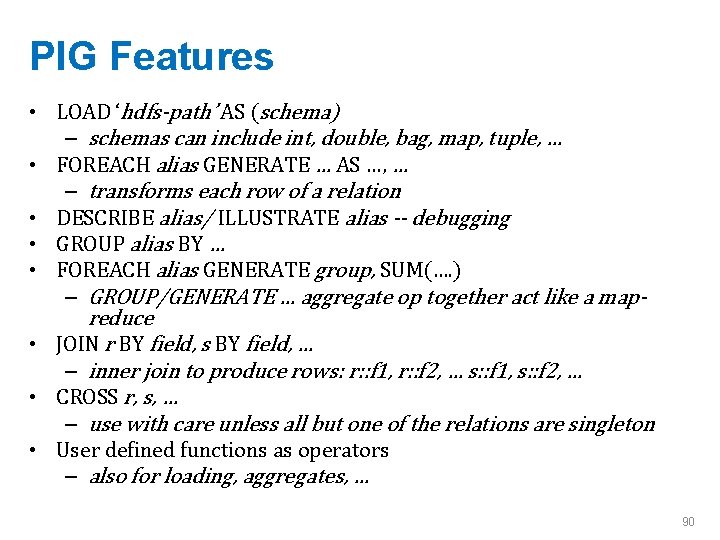
PIG Features • LOAD ‘hdfs-path’ AS (schema) – schemas can include int, double, bag, map, tuple, … • FOREACH alias GENERATE … AS …, … – transforms each row of a relation • DESCRIBE alias/ ILLUSTRATE alias -- debugging • GROUP alias BY … • FOREACH alias GENERATE group, SUM(…. ) – GROUP/GENERATE … aggregate op together act like a mapreduce • JOIN r BY field, s BY field, … – inner join to produce rows: r: : f 1, r: : f 2, … s: : f 1, s: : f 2, … • CROSS r, s, … – use with care unless all but one of the relations are singleton • User defined functions as operators – also for loading, aggregates, … 90

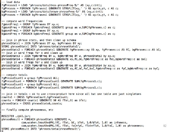
The full phrase-finding pipeline in PIG 91

92