Constrained Exact Optimization in Phylogenetics Tandy Warnow The

Constrained Exact Optimization in Phylogenetics Tandy Warnow The University of Illinois at Urbana-Champaign

Phylogeny (evolutionary tree) Orangutan From the Tree of the Life Website, University of Arizona Gorilla Chimpanzee Human

DNA Sequence Evolution -3 mil yrs AAGACTT AAGGCCT AGGGCAT TAGCCCA TGGACTT TAGCCCT AGCACTT TAGACTT AGCACAA AGCGCTT -2 mil yrs -1 mil yrs today

Phylogeny Problem U AGTGCAT V W TAGCCCA X TAGACTT Y TGCACAA X U Y V W TGCGCTT

Phylogeny + genomics = genome-scale phylogeny estimation.

Species Main competing approaches gene 1 gene 2. . . gene k Concatenation Analyze separately . . . Summary Method

Phylogenomic pipeline • Select taxon set and markers • Gather and screen sequence data, possibly identify orthologs • Compute multiple sequence alignment and “gene tree” for each locus • Compute species tree or phylogenetic network from the gene trees or alignments • Get statistical support on each branch (e. g. , bootstrapping) • Estimate dates on the nodes of the phylogeny • Use species tree with branch support and dates to understand biology

Just about everything worth doing is NP-hard • • Multiple sequence alignment Maximum likelihood gene tree estimation Species tree estimation by combining gene trees Supertree estimation – and hence divide-and-conquer strategies And Bayesian methods are even more computationally intensive

Just about everything worth doing is NP-hard • • Multiple sequence alignment Maximum likelihood gene tree estimation Species tree estimation by combining gene trees Supertree estimation – and hence divide-and-conquer strategies And Bayesian methods are even more computationally intensive

Local search heuristics Figure from Huson 2010 Standard heuristic search: TBR moves through “treespace” Randomness to exit local optima But there are (2 n-5)!! trees on n leaves

Solving maximum likelihood (and other hard optimization problems) is… unlikely # of Taxa # of Unrooted Trees 4 3 5 15 6 105 7 945 8 10395 9 135135 10 2027025 20 2. 2 x 1020 100 4. 5 x 10190 1000 2. 7 x 102900

Only 48 species, but heuristic ML took ~300 CPU years on multiple supercomputers and used 1 Tb of memory

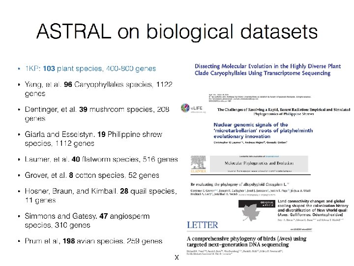
1 KP: Thousand Transcriptome Project G. Ka-Shu Wong J. Leebens-Mack U Georgia U Alberta N. Wickett Northwestern N. Matasci i. Plant T. Warnow, UIUC S. Mirarab, UCSD N. Nguyen UCSD And many others 103 plant transcriptomes, 400 -800 single copy “genes” Wickett, Mirarab et al. , PNAS 2014 Next phase will be much bigger ~1000 species and ~1000 genes, and will require the inference of multiple sequence alignments and trees on more than 100, 000 sequences

Muir, 2016

This Talk • Model-based tree estimation and NP-hard problems • How divide-and-conquer can improve tree estimation • Constrained optimization • Open problems

Markov Model of Site Evolution Simplest (Jukes-Cantor, 1969): • The model tree T is binary and has substitution probabilities p(e) on each edge e. • The state at the root is randomly drawn from {A, C, T, G} (nucleotides) • If a site (position) changes on an edge, it changes with equal probability to each of the remaining states. • The evolutionary process is Markovian. The different sites are assumed to evolve independently and identically down the tree (with rates that are drawn from a gamma distribution). More complex models (such as the General Markov model) are also considered, often with little change to theory.

Questions • Is the model tree identifiable? • Which estimation methods are statistically consistent under this model? • How much data does the method need to estimate the model tree correctly (with high probability), and how well do the methods perform in practice?

Statistical Consistency error Data

Answers? • We know a lot about which site evolution models are identifiable, and which methods are statistically consistent. • We know a little bit about the sequence length requirements for standard methods. • Extensive studies show that even the best methods produce gene trees with some error.

Statistically consistent phylogenetic reconstruction methods 1 Hill-climbing heuristics for NP-hard optimization criteria (e. g. , Maximum Likelihood) Local optimum Cost Global optimum Phylogenetic trees 2 3. Polynomial time distance-based methods: Neighbor Joining, Fast. ME, etc. Bayesian methods

Distance-based estimation

Quantifying Error FN FN: false negative (missing edge) FP: false positive (incorrect edge) 50% error rate FP

Neighbor Joining (NJ) on large trees Error Rate 0. 8 Simulation study based upon fixed edge lengths, K 2 P model of evolution, sequence lengths fixed to 1000 nucleotides. Error rates reflect proportion of incorrect edges in inferred trees. NJ 0. 6 0. 4 0. 2 [Nakhleh et al. ISMB 2001] 0 0 400 800 No. Taxa 1200 1600

In other words… error Data Statistical consistency doesn’t guarantee accuracy w. h. p. unless the sequences are long enough.

“Boosting” phylogeny reconstruction methods • DCMs “boost” the performance of phylogeny reconstruction methods. Base method M DCM-M

Divide-and-conquer for phylogeny estimation

Markov Model of Site Evolution Simplest (Jukes-Cantor, 1969): • The model tree T is binary and has substitution probabilities p(e) on each edge e. • The state at the root is randomly drawn from {A, C, T, G} (nucleotides) • If a site (position) changes on an edge, it changes with equal probability to each of the remaining states. • The evolutionary process is Markovian. The different sites are assumed to evolve independently and identically down the tree (with rates that are drawn from a gamma distribution). More complex models (such as the General Markov model) are also considered, often with little change to theory.

Sequence length requirements The sequence length (number of sites) that a phylogeny reconstruction method M needs to reconstruct the true tree with probability at least 1 - depends on • M (the method) • • f = min p(e), • g = max p(e), and • n, the number of leaves We fix everything but n.

Statistical consistency, exponential convergence, and absolute fast convergence (afc)

Distance-based estimation

Neighbor Joining’s sequence length requirement is exponential! • Atteson 1999: Let T be a Jukes-Cantor model tree defining additive matrix D. Then Neighbor Joining will reconstruct the true tree with high probability from sequences that are of length O(lg n emax Dij). • Lacey and Chang 2009: Matching lower bound

Divide-and-conquer for phylogeny estimation Construct subset trees Supertree Step Refinement Step

DCM 1 Decompositions Input: Set S of sequences, distance matrix d, threshold value 1. Compute threshold graph 2. Perform minimum weight triangulation (note: if d is an additive matrix, then the threshold graph is provably triangulated). DCM 1 decomposition : Compute maximal cliques

DCM 1 -boosting: Warnow, St. John, and Moret, SODA 2001 Exponentially converging (base) method DCM 1 SQS Absolute fast converging (DCM 1 -boosted) method • The DCM 1 phase produces a collection of trees (one for each threshold), and the SQS phase picks the “best” tree. • For a given threshold, the base method is used to construct trees on small subsets (defined by the threshold) of the taxa. These small trees are then combined into a tree on the full set of taxa.

Neighbor Joining on large diameter trees Error Rate 0. 8 Simulation study based upon fixed edge lengths, K 2 P model of evolution, sequence lengths fixed to 1000 nucleotides. Error rates reflect proportion of incorrect edges in inferred trees. NJ 0. 6 0. 4 0. 2 [Nakhleh et al. ISMB 2001] 0 0 400 800 No. Taxa 1200 1600

DCM 1 -boosting distance-based methods [Nakhleh et al. ISMB 2001] Error Rate 0. 8 NJ DCM 1 -NJ 0. 6 0. 4 • Theorem (Warnow et al. , SODA 2001): DCM 1 -NJ converges to the true tree from polynomial length sequences 0. 2 0 0 400 800 No. Taxa 1200 1600

DCM 1 -boosting • DCM 1 -boosting: reducing sequence length requirements for gene tree accuracy from exponential to polynomial • Key algorithmic ingredients: – Construct triangulated graph – Apply tree construction methods to subsets – Combine subset trees together using supertree method – Select best tree from a set of trees

DCM 1 -boosting • DCM 1 -boosting: reducing sequence length requirements for gene tree accuracy from exponential to polynomial • Key algorithmic ingredients: – Construct triangulated graph – Apply tree construction methods to subsets – Combine subset trees together using supertree method – Select best tree from a set of trees

Other applications of divide-and-conquer • DACTAL-boosting: – almost alignment-free tree estimation – Improving multi-locus species tree estimation • DCM 2 -boosting: improving heuristic searches for maximum likelihood • Superfine-boosting: improving supertree methods

Divide-and-conquer for phylogeny estimation Construct subset trees Supertree Step Refinement Step

Supertree Problems • • • Quartet Median Supertree Robinson-Foulds Supertree Matrix Representation with Parsimony Matrix Representation with Likelihood Etc. All are NP-hard because even testing compatibility of unrooted trees is NP-complete.

Supertree Problems • • • Quartet Median Supertree Robinson-Foulds Supertree Matrix Representation with Parsimony Matrix Representation with Likelihood Etc. All are NP-hard because even testing compatibility of unrooted trees is NP-complete.

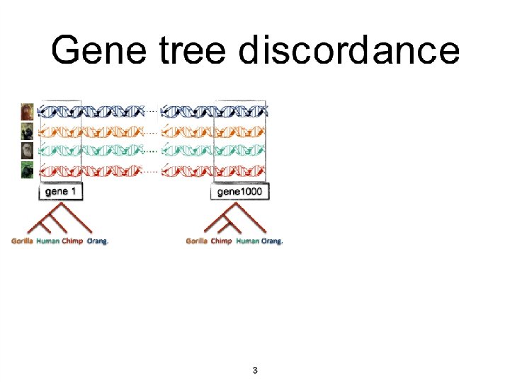
Incomplete Lineage Sorting (ILS) is a dominant cause of gene tree heterogeneity

Gene trees inside the species tree (Coalescent Process) Past Present Courtesy James Degnan Gorilla and Orangutan are not siblings in the species tree, but they are in the gene tree.

Incomplete Lineage Sorting (ILS) • Confounds phylogenetic analysis for many groups: Hominids, Birds, Yeast, Animals, Toads, Fish, Fungi, etc. • There is substantial debate about how to analyze phylogenomic datasets in the presence of ILS, focused around statistical consistency guarantees (theory) and performance on data.

Anomaly zone • An anomalous gene tree (AGT) is one that is more probable than the true species tree under the multispecies coalescent model. • Theorem (Hudson 1983): There are no rooted 3 -leaf AGTs. • Theorem (Allman et al. 2011, Degnan 2013): There are no unrooted 4 -leaf AGTs. • Theorem (Degnan 2013, Rosenberg 2013): For n>3, there are model species trees with rooted AGTs, and for n>4 there are model species trees with unrooted AGTs.

Anomaly zone • An anomalous gene tree (AGT) is one that is more probable than the true species tree under the multispecies coalescent model. • Theorem (Hudson 1983): There are no rooted 3 -leaf AGTs. • Theorem (Allman et al. 2011, Degnan 2013): There are no unrooted 4 -leaf AGTs. • Theorem (Degnan 2013, Rosenberg 2013): For n>3, there are model species trees with rooted AGTs, and for n>4 there are model species trees with unrooted AGTs.

Anomaly zone • An anomalous gene tree (AGT) is one that is more probable than the true species tree under the multispecies coalescent model. • Theorem (Hudson 1983): There are no rooted 3 -leaf AGTs. • Theorem (Allman et al. 2011, Degnan 2013): There are no unrooted 4 -leaf AGTs. • Theorem (Degnan 2013, Rosenberg 2013): For n>3, there are model species trees with rooted AGTs, and for n>4 there are model species trees with unrooted AGTs.

Anomaly zone • An anomalous gene tree (AGT) is one that is more probable than the true species tree under the multispecies coalescent model. • Theorem (Hudson 1983): There are no rooted 3 -leaf AGTs. • Theorem (Allman et al. 2011, Degnan 2013): There are no unrooted 4 -leaf AGTs. • Theorem (Degnan 2013, Rosenberg 2013): For n>3, there are model species trees with rooted AGTs, and for n>4 there are model species trees with unrooted AGTs.

Anomaly zone • An anomalous gene tree (AGT) is one that is more probable than the true species tree under the multispecies coalescent model. • Theorem (Hudson 1983): There are no rooted 3 -leaf AGTs. • Theorem (Allman et al. 2011, Degnan 2013): There are no unrooted 4 -leaf AGTs. • Theorem (Degnan 2013, Rosenberg 2013): For n>3, there are model species trees with rooted AGTs, and for n>4 there are model species trees with unrooted AGTs.

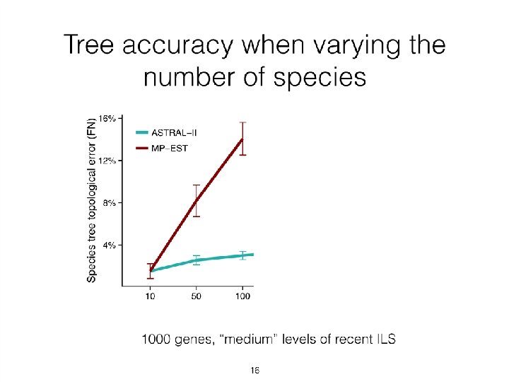
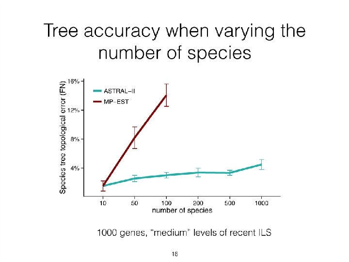
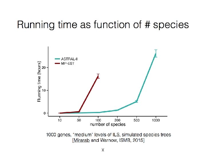
Constrained Maximum Quartet Support Tree • Input: Set T = {t 1, t 2, …, tk} of unrooted gene trees, with each tree on set S with n species, and set X of allowed bipartitions • Output: Unrooted tree T on leafset S, maximizing the total quartet tree similarity to T, subject to T drawing its bipartitions from X. Theorems: • Mirarab et al. 2014: If X contains the bipartitions from the input gene trees (and perhaps others), then an exact solution to this problem is statistically consistent under the MSC. • Mirarab and Warnow 2015: The constrained MQST problem can be solved in O(|X|2 nk) time. (We use dynamic programming, and build the unrooted tree from the bottom-up, based on “allowed clades” – halves of the allowed bipartitions. )

Constrained Maximum Quartet Support Tree • Input: Set T = {t 1, t 2, …, tk} of unrooted gene trees, with each tree on set S with n species, and set X of allowed bipartitions • Output: Unrooted tree T on leafset S, maximizing the total quartet tree similarity to T, subject to T drawing its bipartitions from X. Theorems: • Mirarab et al. 2014: If X contains the bipartitions from the input gene trees (and perhaps others), then an exact solution to this problem is statistically consistent under the MSC. • Mirarab and Warnow 2015: The constrained MQST problem can be solved in O(|X|2 nk) time. (We use dynamic programming, and build the unrooted tree from the bottom-up, based on “allowed clades” – halves of the allowed bipartitions. )

Constrained Maximum Quartet Support Tree • Input: Set T = {t 1, t 2, …, tk} of unrooted gene trees, with each tree on set S with n species, and set X of allowed bipartitions • Output: Unrooted tree T on leafset S, maximizing the total quartet tree similarity to T, subject to T drawing its bipartitions from X. Theorems: • Mirarab et al. 2014: If X contains the bipartitions from the input gene trees (and perhaps others), then an exact solution to this problem is statistically consistent under the MSC. • Mirarab and Warnow 2015: The constrained MQST problem can be solved in O(|X|2 nk) time. (We use dynamic programming, and build the unrooted tree from the bottom-up, based on “allowed clades” – halves of the allowed bipartitions. )

Used Sim. Phy, Mallo and Posada, 2015

Other polynomial time algorithms for constrained optimization problems • Minimize Duplication/Loss Supertree (Hallett and Lagergren 2000) • Quartet Support (Bryant and Steel 2001) • Constrained Minimize Deep Coalescence (Than and Nakhleh 2000, Yu, Warnow, and Nakhleh 2011). • Gene tree estimation under Duplication and Loss (Szöllősi et al. 2013) • Constrained Robinson-Foulds Supertree (Vachaspati and Warnow 2016)

Summary • NP-hard optimization problems abound in phylogeny reconstruction, and in computational biology in general, and need very accurate solutions. • Divide-and-conquer techniques can provide greatly improved accuracy and scalability, and excellent statistical performance guarantees. But divide-andconquer methods depend on having good supertree methods. • Constrained exact optimization has been surprisingly beneficial for phylogenomic analysis.

Summary • NP-hard optimization problems abound in phylogeny reconstruction, and in computational biology in general, and need very accurate solutions. • Divide-and-conquer techniques can provide greatly improved accuracy and scalability, and excellent statistical performance guarantees. But divide-andconquer methods depend on having good supertree methods. • Constrained exact optimization has been surprisingly beneficial for phylogenomic analysis.

Summary • NP-hard optimization problems abound in phylogeny reconstruction, and in computational biology in general, and need very accurate solutions. • Divide-and-conquer techniques can provide greatly improved accuracy and scalability, and excellent statistical performance guarantees. But divide-andconquer methods depend on having good supertree methods. • Constrained exact optimization has been surprisingly beneficial for phylogenomic analysis.

Open Problems • What other optimization problems are tractable, given constraint sets? • How should we define the set X of constraints from a set of source trees, especially when the source trees are incomplete? • Are there other ways of constraining the search space that are effective and useful? • What are other effective ways of approaching truly largescale phylogeny estimation? • Can divide-and-conquer be employed with Bayesian methods? (Or, more generally, how can we make Bayesian methods more scalable? )

Acknowledgments NSF grant DBI-1461364 (joint with Noah Rosenberg at Stanford and Luay Nakhleh at Rice): http: //tandy. cs. illinois. edu/Phylogenomics. Project. html Papers available at http: //tandy. cs. illinois. edu/papers. html ASTRAL: Available at https: //github. com/smirarab Fast. RFS: Available at https: //github. com/pranjalv 123/Fast. RFS

Constrained Robinson-Foulds Supertree • Input: set T of source trees, and set X of allowed bipartitions • Output: tree T that minimizes the total Robinson. Foulds distance to the input source trees, and that draws its bipartitions from X. Theorem (Vachaspati and Warnow 2016): The onstrained RF Supertree can be solved in O(|X|2 nk) time, where there are k source trees and n species.

Constrained optimization • First proposed in Hallet and Lagergren 2000, for the duplication-loss species tree problem • Algorithms for constrained optimization use dynamic programming to find optimal solutions, constructing the best tree from the “bottom-up” • The set X is usually defined to be the bipartitions from the source trees.

Triangulated Graphs • Definition: A graph is triangulated if it has no simple cycles of size four or more.

Sampling multiple genes from multiple species Orangutan From the Tree of the Life Website, University of Arizona Gorilla Chimpanzee Human

Standard heuristic search T Random perturbation Hill-climbing T’

Problems with current techniques for MP Shown here is the performance of the TNT software for maximum parsimony on a real dataset of almost 14, 000 sequences. The required level of accuracy with respect to MP score is no more than 0. 01% error (otherwise high topological error results). (“Optimal” here means best score to date, using any method for any amount of time. ) Performance of TNT with time

Solving NP-hard problems exactly is … unlikely • Number of (unrooted) binary trees on n leaves is (2 n-5)!! • If each tree on 1000 taxa could be analyzed in 0. 001 seconds, we would find the best tree in 2890 millennia #leaves #trees 4 3 5 15 6 105 7 945 8 10395 9 135135 10 2027025 20 2. 2 x 1020 100 4. 5 x 10190 1000 2. 7 x 102900

Avian Phylogenomics Project Plus many other people… E Jarvis, HHMI MTP Gilbert, Copenhagen G Zhang, BGI T. Warnow UT-Austin S. Mirarab Md. S. Bayzid, UT-Austin • Approx. 50 species, whole genomes, 14, 000 loci Challenges: • Concatenation analysis used >200 CPU years But also • Massive gene tree conflict suggestive of ILS, and most gene trees had very low bootstrap support • Coalescent-based analysis using MP-EST produced tree that conflicted with concatenation analysis

Big datasets and hard problems • Computationally intensive problems: – Multiple sequence alignment – Maximum likelihood gene tree estimation – Species tree estimation from multiple gene trees • Fast methods are generally not sufficiently accurate • Accurate methods are generally computationally intensive

Quantifying Error FN FN: false negative (missing edge) FP: false positive (incorrect edge) 50% error rate FP

Neighbor joining has poor performance on large diameter trees [Nakhleh et al. ISMB 2001] 0. 8 NJ Error Rate Theorem (Atteson): Exponential sequence length requirement for Neighbor Joining! 0. 6 0. 4 0. 2 0 0 400 800 No. Taxa 1200 1600

Species Tree Estimation requires multiple genes! Orangutan From the Tree of the Life Website, University of Arizona Gorilla Chimpanzee Human

Species tree estimation: difficult, even for small datasets! Orangutan From the Tree of the Life Website, University of Arizona Gorilla Chimpanzee Human

Major Challenges: large datasets, fragmentary sequences • Multiple sequence alignment: Few methods can run on large datasets, and alignment accuracy is generally poor for large datasets with high rates of evolution. • Gene Tree Estimation: standard methods have poor accuracy on even moderately large datasets, and the most accurate methods are enormously computationally intensive (weeks or months, high memory requirements). • Species Tree Estimation: gene tree incongruence makes accurate estimation of species tree challenging. • Phylogenetic Network Estimation: Horizontal gene transfer and hybridization requires non-tree models of evolution Both phylogenetic estimation and multiple sequence alignment are also impacted by fragmentary data.

Major Challenges: large datasets, fragmentary sequences • Multiple sequence alignment: Few methods can run on large datasets, and alignment accuracy is generally poor for large datasets with high rates of evolution. • Gene Tree Estimation: standard methods have poor accuracy on even moderately large datasets, and the most accurate methods are enormously computationally intensive (weeks or months, high memory requirements). • Species Tree Estimation: gene tree incongruence makes accurate estimation of species tree challenging. • Phylogenetic Network Estimation: Horizontal gene transfer and hybridization requires non-tree models of evolution Both phylogenetic estimation and multiple sequence alignment are also impacted by fragmentary data.

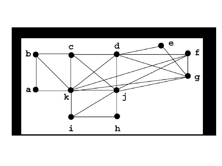
Strict Consensus Merger (SCM) b e a f c a d g b e a c f b g h h i j d i j f c c c b d b a e a d h i j g d

The Tree of Life: Multiple Challenges Large datasets: 100, 000+ sequences 10, 000+ genes “Big. Data” complexity Large-scale statistical phylogeny estimation Ultra-large multiple-sequence alignment Estimating species trees from incongruent gene trees Supertree estimation Genome rearrangement phylogeny Reticulate evolution Visualization of large trees and alignments Data mining techniques to explore multiple optima

The Tree of Life: Multiple Challenges Scientific challenges: • • • Ultra-large multiple-sequence alignment Alignment-free phylogeny estimation Supertree estimation Estimating species trees from many gene trees Genome rearrangement phylogeny Reticulate evolution Visualization of large trees and alignments Data mining techniques to explore multiple optima Theoretical guarantees under Markov models of evolution Applications: • • • metagenomics protein structure and function prediction trait evolution detection of co-evolution systems biology Techniques: • • • Graph theory (especially chordal graphs) Probability theory and statistics Hidden Markov models Combinatorial optimization Heuristics Supercomputing

1 kp: Thousand Transcriptome Project G. Ka-Shu Wong U Alberta J. Leebens-Mack U Georgia N. Wickett Northwestern N. Matasci i. Plant T. Warnow, UIUC S. Mirarab, UT-Austin N. Nguyen, UT-Austin Plus many other people… Plant Tree of Life based on transcriptomes of ~1200 species More than 13, 000 gene families (most not single copy) First paper: PNAS 2014 (~100 species and ~800 loci) • Gene Tree Incongruence Upcoming Challenges (~1200 species, ~400 loci): • Species tree estimation under the multi-species coalescent from hundreds of conflicting gene trees on >1000 species (we will use ASTRAL – Mirarab et al. 2014, Mirarab & Warnow 2015) • Multiple sequence alignment of >100, 000 sequences (with lots of fragments!) – we will use UPP (Nguyen et al. , 2015)