Rational Choice CHOICE 1 2 Scarcity income constraint

Rational Choice

CHOICE 1. 2. Scarcity (income constraint) Tastes (indifference map/utility function)

ECONOMIC RATIONALITY u The principal behavioral postulate is that a decision-maker chooses its most preferred alternative from those available to it. u The available choices constitute the choice set. u How is the most preferred bundle in the choice set located/found?

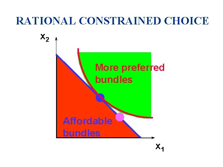
RATIONAL CONSTRAINED CHOICE x 2 More preferred bundles Affordable bundles x 1

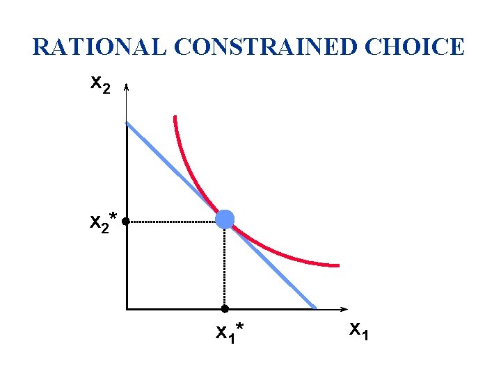
RATIONAL CONSTRAINED CHOICE x 2* x 1

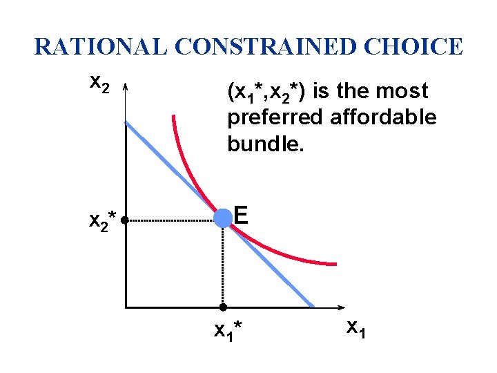
RATIONAL CONSTRAINED CHOICE x 2 (x 1*, x 2*) is the most preferred affordable bundle. x 2* E x 1* x 1

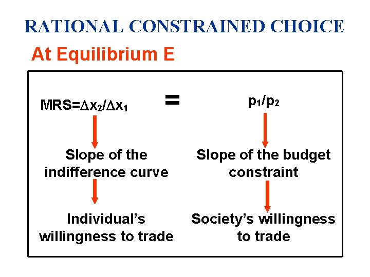
RATIONAL CONSTRAINED CHOICE At Equilibrium E MRS= x 2/ x 1 = p 1/p 2 Slope of the indifference curve Slope of the budget constraint Individual’s willingness to trade Society’s willingness to trade

RATIONAL CONSTRAINED CHOICE u The most preferred affordable bundle is called the consumer’s ORDINARY DEMAND at the given prices and income. u Ordinary demands will be denoted by x 1*(p 1, p 2, m) and x 2*(p 1, p 2, m).

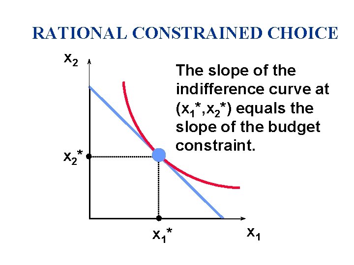
RATIONAL CONSTRAINED CHOICE x 2 The slope of the indifference curve at (x 1*, x 2*) equals the slope of the budget constraint. x 2* x 1

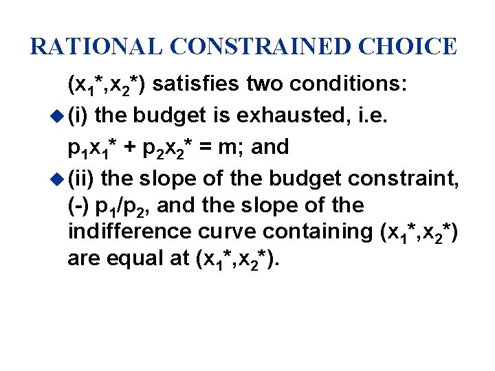
RATIONAL CONSTRAINED CHOICE (x 1*, x 2*) satisfies two conditions: u (i) the budget is exhausted, i. e. p 1 x 1* + p 2 x 2* = m; and u (ii) the slope of the budget constraint, (-) p 1/p 2, and the slope of the indifference curve containing (x 1*, x 2*) are equal at (x 1*, x 2*).

COMPUTING DEMAND u u 1. 2. How can this information be used to locate (x 1*, x 2*) for given p 1, p 2 and m? Two ways to do this Use Lagrange multiplier method Find MRS and substitute into the Budget Constraint

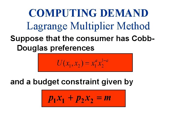
COMPUTING DEMAND Lagrange Multiplier Method Suppose that the consumer has Cobb. Douglas preferences and a budget constraint given by

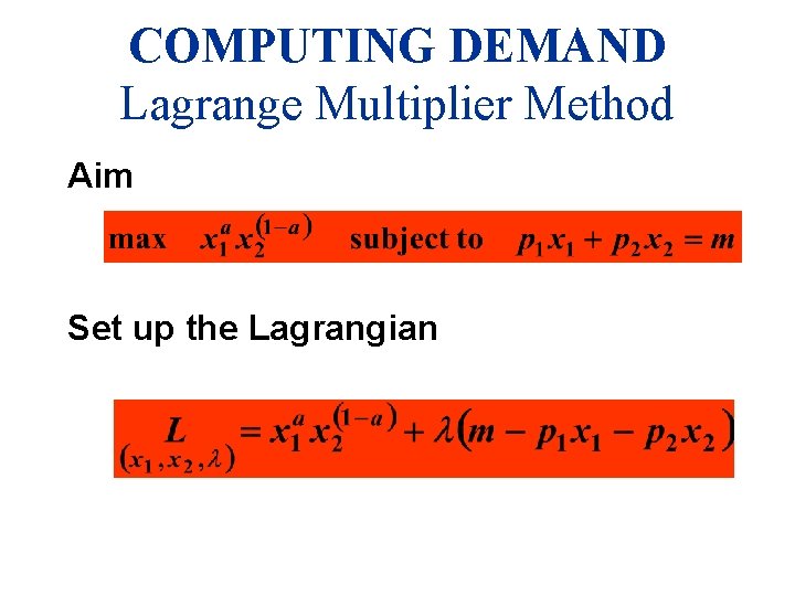
COMPUTING DEMAND Lagrange Multiplier Method Aim Set up the Lagrangian

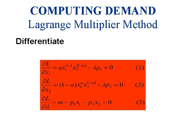
COMPUTING DEMAND Lagrange Multiplier Method Differentiate

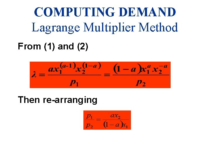
COMPUTING DEMAND Lagrange Multiplier Method From (1) and (2) Then re-arranging

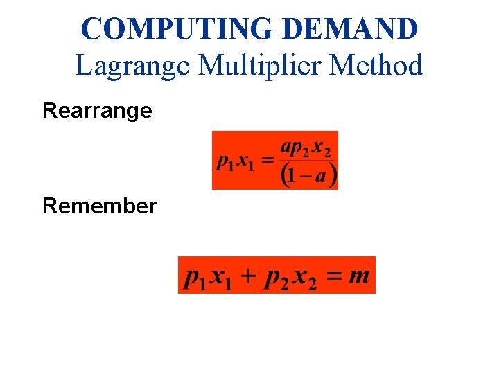
COMPUTING DEMAND Lagrange Multiplier Method Rearrange Remember

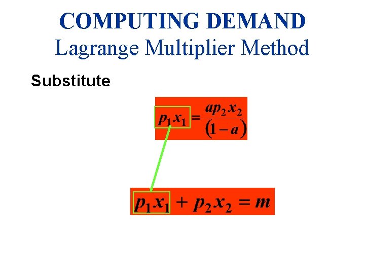
COMPUTING DEMAND Lagrange Multiplier Method Substitute

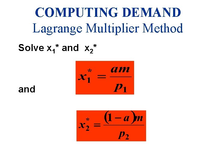
COMPUTING DEMAND Lagrange Multiplier Method Solve x 1* and x 2* and

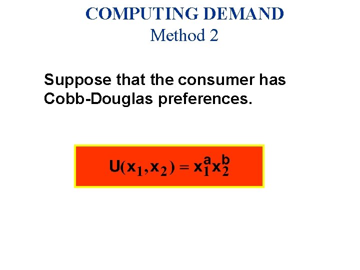
COMPUTING DEMAND Method 2 Suppose that the consumer has Cobb-Douglas preferences.

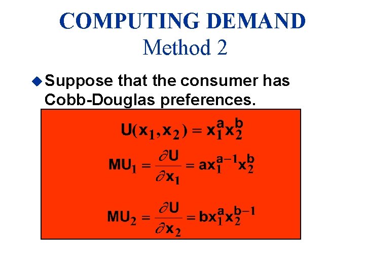
COMPUTING DEMAND Method 2 u Suppose that the consumer has Cobb-Douglas preferences.

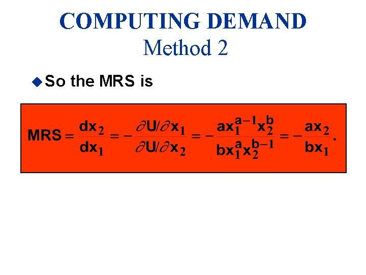
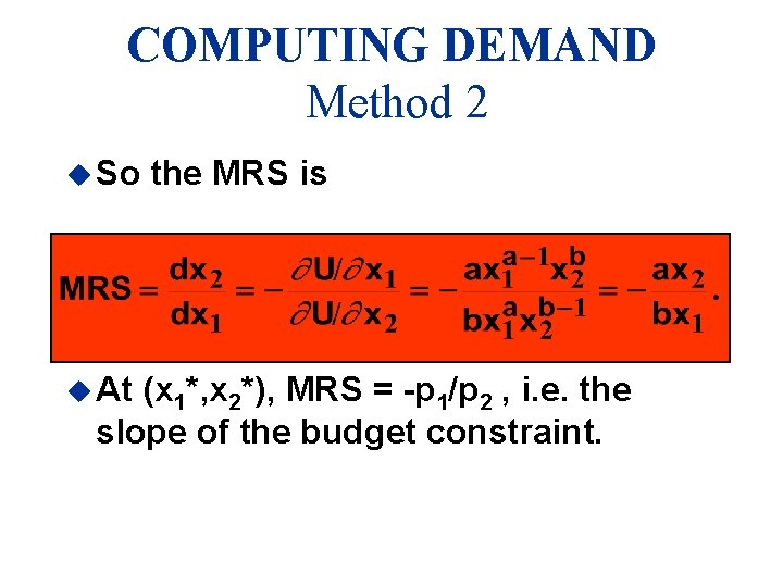
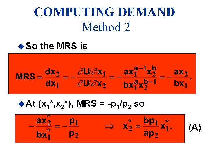
COMPUTING DEMAND Method 2 u So the MRS is

COMPUTING DEMAND Method 2 u So u At the MRS is (x 1*, x 2*), MRS = -p 1/p 2 , i. e. the slope of the budget constraint.

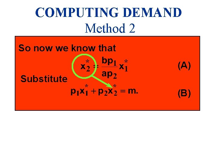
COMPUTING DEMAND Method 2 u So the MRS is u At (x 1*, x 2*), MRS = -p 1/p 2 so (A)

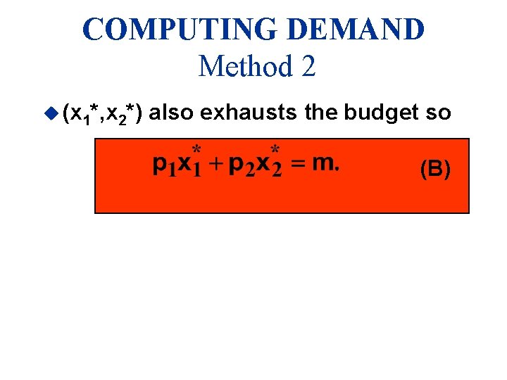
COMPUTING DEMAND Method 2 u (x 1*, x 2*) also exhausts the budget so (B)

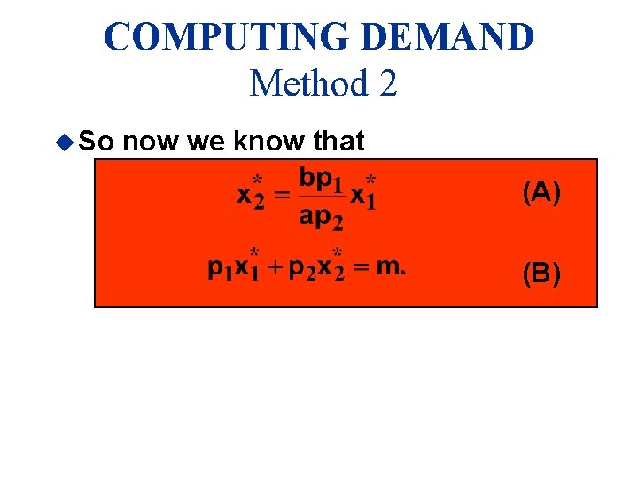
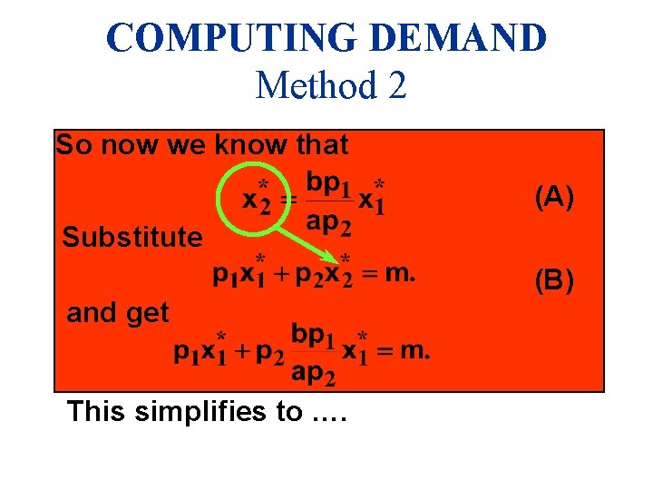
COMPUTING DEMAND Method 2 u So now we know that (A) (B)

COMPUTING DEMAND Method 2 So now we know that (A) Substitute (B)

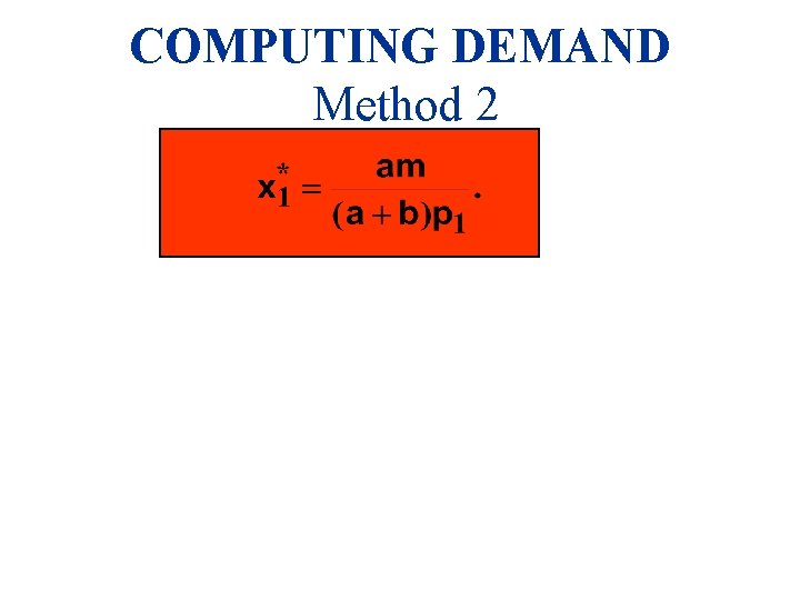
COMPUTING DEMAND Method 2 So now we know that (A) Substitute and get This simplifies to …. (B)

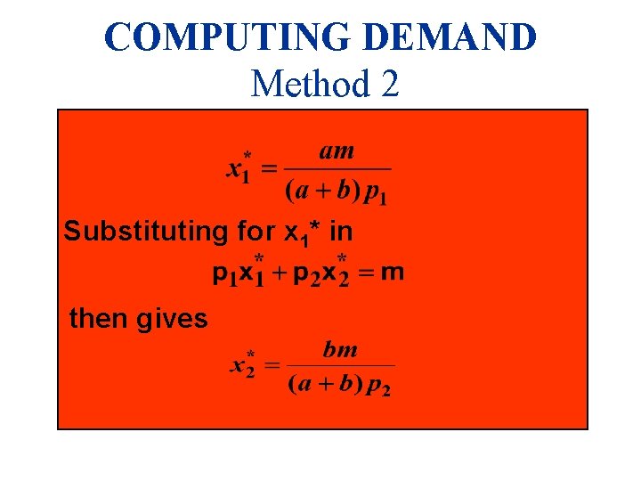
COMPUTING DEMAND Method 2

COMPUTING DEMAND Method 2 Substituting for x 1* in then gives

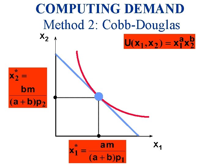
COMPUTING DEMAND Method 2 So we have discovered that the most preferred affordable bundle for a consumer with Cobb-Douglas preferences is

COMPUTING DEMAND Method 2: Cobb-Douglas x 2 x 1

Rational Constrained Choice u But what if x 1* = 0 or x 2* = 0? u If either x 1* = 0 or x 2* = 0 then the ordinary demand (x 1*, x 2*) is at a corner solution to the problem of maximizing utility subject to a budget constraint.

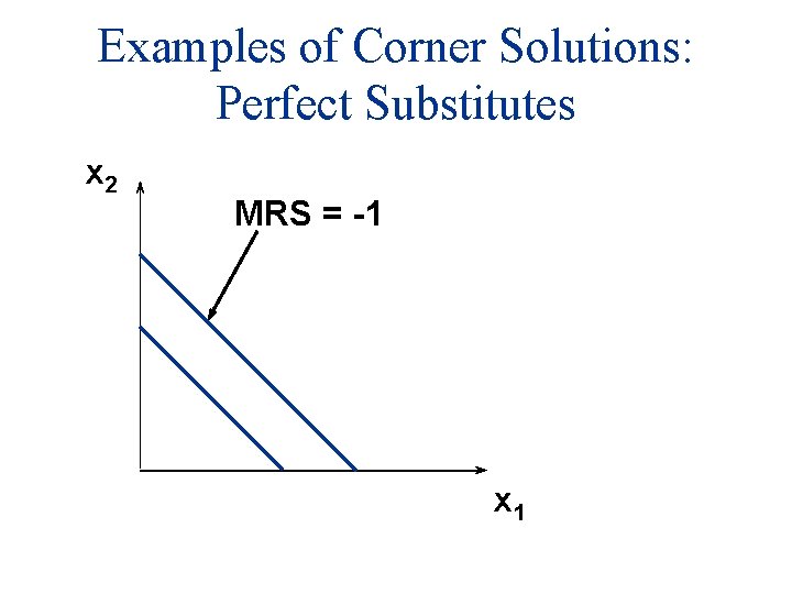
Examples of Corner Solutions: Perfect Substitutes x 2 MRS = -1 x 1

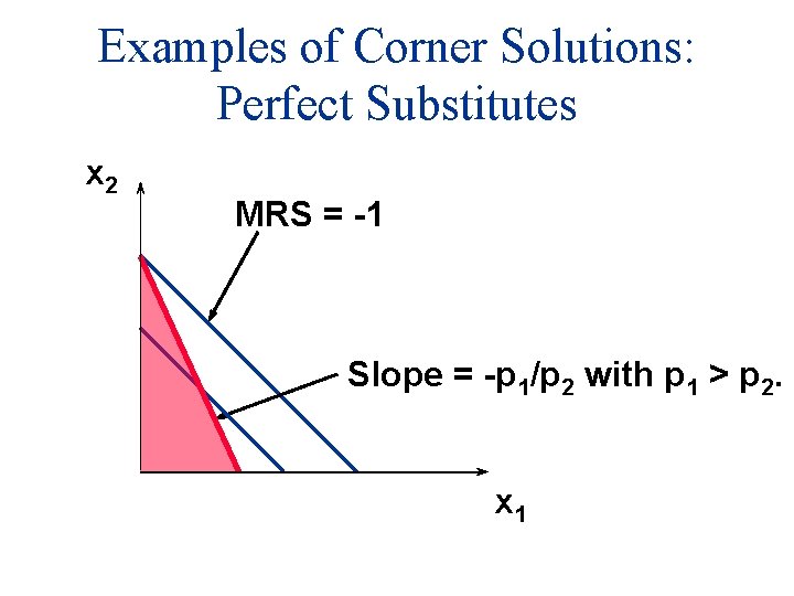
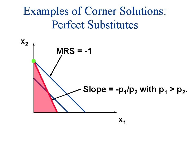
Examples of Corner Solutions: Perfect Substitutes x 2 MRS = -1 Slope = -p 1/p 2 with p 1 > p 2. x 1

Examples of Corner Solutions: Perfect Substitutes x 2 MRS = -1 Slope = -p 1/p 2 with p 1 > p 2. x 1

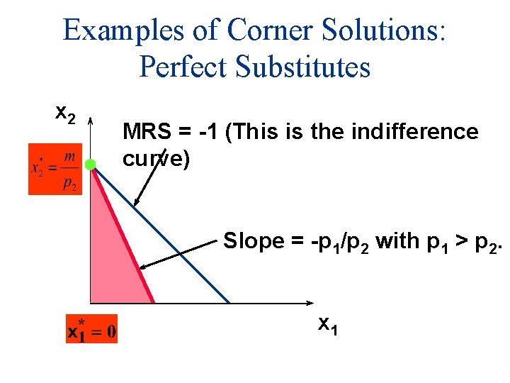
Examples of Corner Solutions: Perfect Substitutes x 2 MRS = -1 (This is the indifference curve) Slope = -p 1/p 2 with p 1 > p 2. x 1

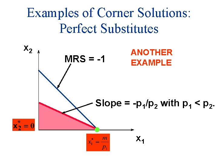
Examples of Corner Solutions: Perfect Substitutes x 2 MRS = -1 ANOTHER EXAMPLE Slope = -p 1/p 2 with p 1 < p 2. x 1

Examples of Corner Solutions: Perfect Substitutes So when U(x 1, x 2) = x 1 + x 2, the most preferred affordable bundle is (x 1*, x 2*) where if p 1 < p 2 or if p 1 > p 2.

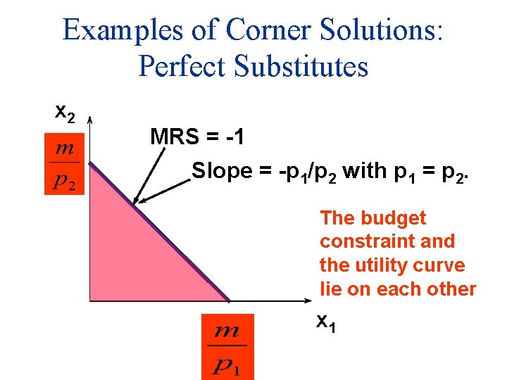
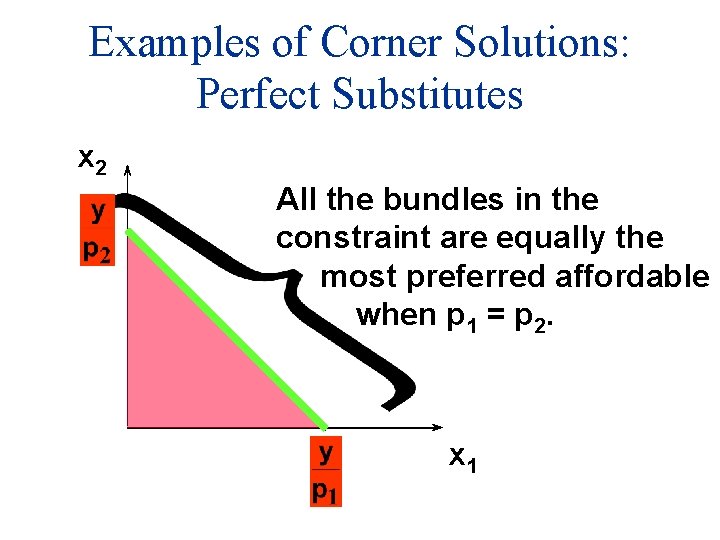
Examples of Corner Solutions: Perfect Substitutes x 2 MRS = -1 Slope = -p 1/p 2 with p 1 = p 2. The budget constraint and the utility curve lie on each other x 1

Examples of Corner Solutions: Perfect Substitutes x 2 All the bundles in the constraint are equally the most preferred affordable when p 1 = p 2. x 1

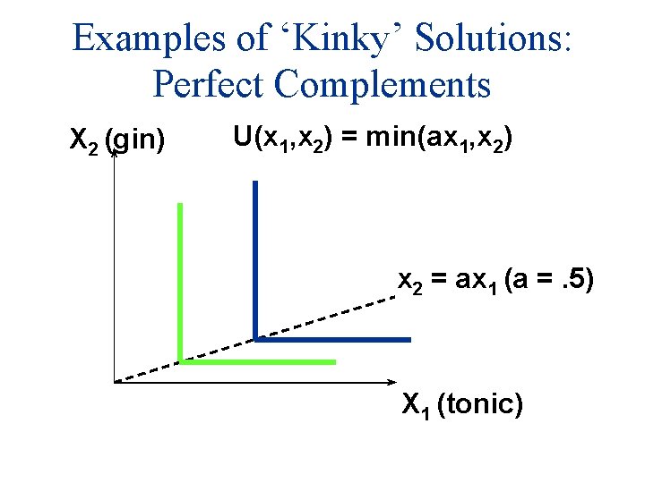
Examples of ‘Kinky’ Solutions: Perfect Complements X 2 (gin) U(x 1, x 2) = min(ax 1, x 2) x 2 = ax 1 (a =. 5) X 1 (tonic)

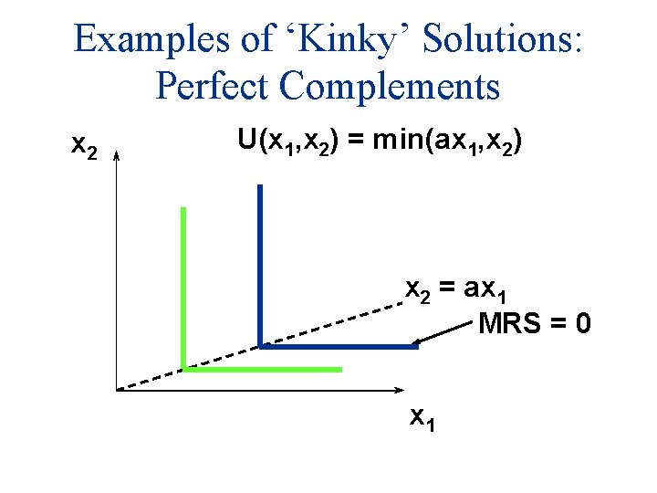
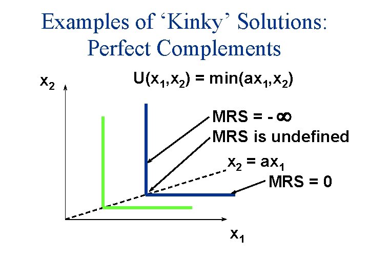
Examples of ‘Kinky’ Solutions: Perfect Complements x 2 U(x 1, x 2) = min(ax 1, x 2) x 2 = ax 1 MRS = 0 x 1

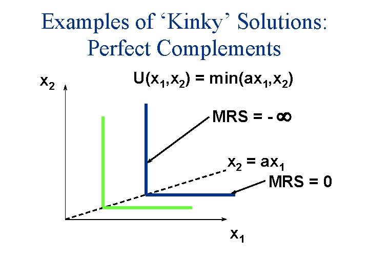
Examples of ‘Kinky’ Solutions: Perfect Complements x 2 U(x 1, x 2) = min(ax 1, x 2) MRS = - ¥ x 2 = ax 1 MRS = 0 x 1

Examples of ‘Kinky’ Solutions: Perfect Complements x 2 U(x 1, x 2) = min(ax 1, x 2) MRS = - ¥ MRS is undefined x 2 = ax 1 MRS = 0 x 1

Examples of ‘Kinky’ Solutions: Perfect Complements x 2 U(x 1, x 2) = min(ax 1, x 2) x 2 = ax 1

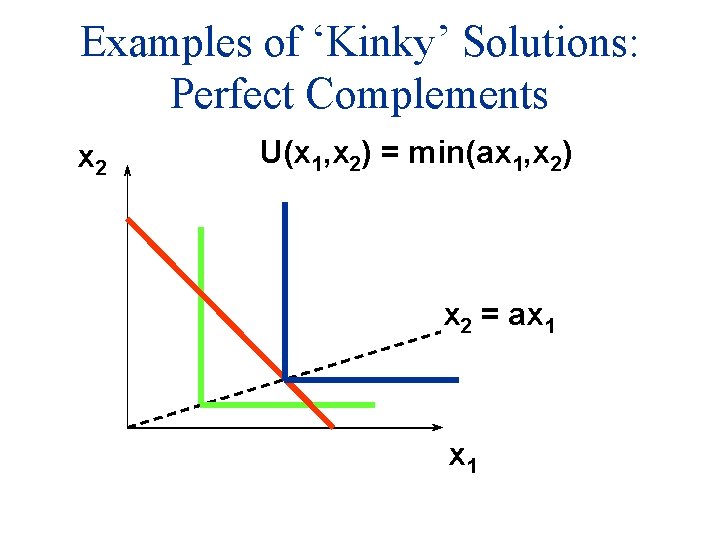
Examples of ‘Kinky’ Solutions: Perfect Complements x 2 U(x 1, x 2) = min(ax 1, x 2) Which is the most preferred affordable bundle? x 2 = ax 1

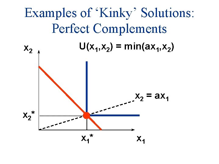
Examples of ‘Kinky’ Solutions: Perfect Complements x 2 U(x 1, x 2) = min(ax 1, x 2) The most preferred affordable bundle x 2 = ax 1

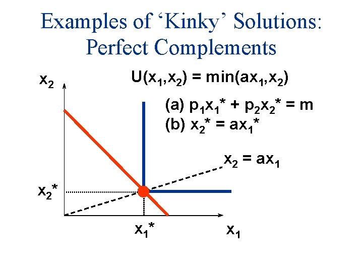
Examples of ‘Kinky’ Solutions: Perfect Complements x 2 U(x 1, x 2) = min(ax 1, x 2) x 2 = ax 1 x 2* x 1

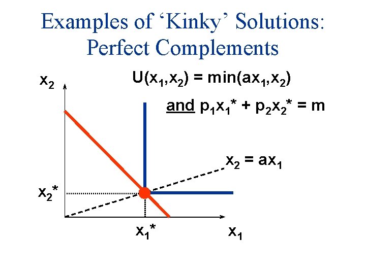
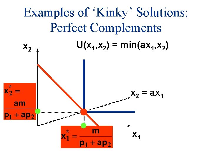
Examples of ‘Kinky’ Solutions: Perfect Complements x 2 U(x 1, x 2) = min(ax 1, x 2) and p 1 x 1* + p 2 x 2* = m x 2 = ax 1 x 2* x 1

Examples of ‘Kinky’ Solutions: Perfect Complements x 2 U(x 1, x 2) = min(ax 1, x 2) (a) p 1 x 1* + p 2 x 2* = m (b) x 2* = ax 1* x 2 = ax 1 x 2* x 1

Examples of ‘Kinky’ Solutions: Perfect Complements (a) p 1 x 1* + p 2 x 2* = m; (b) x 2* = ax 1*

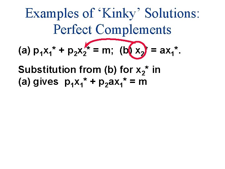
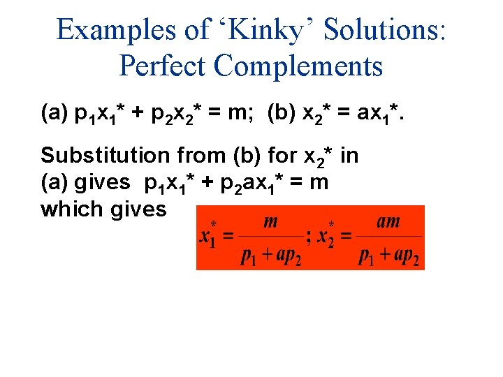
Examples of ‘Kinky’ Solutions: Perfect Complements (a) p 1 x 1* + p 2 x 2* = m; (b) x 2* = ax 1*. Substitution from (b) for x 2* in (a) gives p 1 x 1* + p 2 ax 1* = m

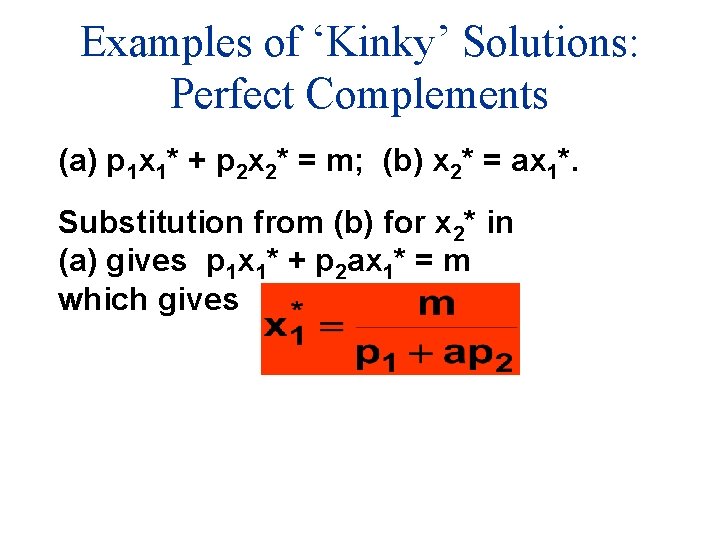
Examples of ‘Kinky’ Solutions: Perfect Complements (a) p 1 x 1* + p 2 x 2* = m; (b) x 2* = ax 1*. Substitution from (b) for x 2* in (a) gives p 1 x 1* + p 2 ax 1* = m which gives

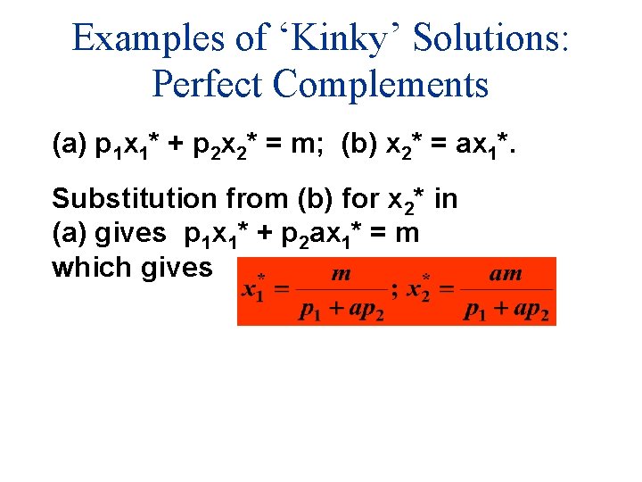
Examples of ‘Kinky’ Solutions: Perfect Complements (a) p 1 x 1* + p 2 x 2* = m; (b) x 2* = ax 1*. Substitution from (b) for x 2* in (a) gives p 1 x 1* + p 2 ax 1* = m which gives

Examples of ‘Kinky’ Solutions: Perfect Complements (a) p 1 x 1* + p 2 x 2* = m; (b) x 2* = ax 1*. Substitution from (b) for x 2* in (a) gives p 1 x 1* + p 2 ax 1* = m which gives

Examples of ‘Kinky’ Solutions: Perfect Complements x 2 U(x 1, x 2) = min(ax 1, x 2) x 2 = ax 1