CS 581 Tandy Warnow This week Maximum parsimony

CS 581 Tandy Warnow

This week • Maximum parsimony: solving it on small datasets • Maximum Likelihood optimization problem • Felsenstein’s pruning algorithm • Bayesian MCMC methods • Research opportunities

Maximum Parsimony • How to solve Maximum Parsimony (MP) on small datasets • MP is statistically consistent on some CFN model trees. • There are some other CFN model trees in which MP is not statistically consistent. • Worse, MP is positively misleading on some CFN model trees (what does this mean? ). – This phenomenon is called “long branch attraction”, and the trees for which MP is not consistent are referred to as “Felsenstein Zone trees” (after the paper by Felsenstein). – The problem is not limited to 4 -leaf trees, and it’s also not limited to CFN. (True also for all standard DNA models. )

Solving MP on small datasets • When the dataset is small enough, you may be able to solve MP (i. e. , find all the best trees) by hand. • Remember: parsimony informative sites • Class exercise: solve MP on datasets

Solving MP on larger datasets • When the dataset is too large, you won’t be able to solve MP by hand • Remember: Fitch algorithm, Sankoff algorithm • Software: PAUP*, TNT, others

Maximum Likelihood Phylogeny Estimation • Maximum Likelihood (ML) is always under a specified model (such as Jukes-Cantor, GTR, CFN, etc. ): – Given the sequence alignment, find the model tree that is most likely to generate the input alignment • This can also be applied to other types of models (i. e. , not just phylogeny estimation given a multiple sequence alignment)

Cavender-Farris-Neyman (CFN) • Models binary sequence evolution • For each edge e, there is a probability p(e) of the property “changing state” (going from 0 to 1, or vice-versa), with 0<p(e)<0. 5 (to ensure that unrooted CFN tree topologies are identifiable). • State at the root is 0 or 1 with equal probability. • Every position evolves under the same process, independently of the others.

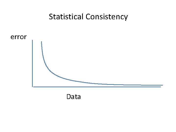
Statistical Consistency error Data

Proving Statistical Consistency under CFN • To prove that a method is statistically consistent under CFN, you have to show: – For all model CFN trees, as the sequence length increases the probability that the method returns the model tree converges to 1. 0. • To prove that a method is not statistically consistent, you only need to find one model CFN tree for which this statement doesn’t hold.

Proving Statistical Consistency under CFN • Some distance-based methods (e. g. , the Naïve Quartet Method) are statistically consistent under the CFN model: – For all model CFN trees, as the sequence length increases the probability that the method returns the model tree converges to 1. 0. • But this isn’t true for Maximum Parsimony or UPGMA (as we showed earlier). • It is true for Maximum Likelihood (we won’t prove this).

Maximum likelihood (ML) under Cavender-Farris-Neyman • Given a set S of binary sequences, find the Cavender-Farris. Neyman model tree (tree topology and substitution probabilities on the edges) that maximizes the probability of producing the input data S. ML, if solved exactly, is statistically consistent under Cavender. Farris (and under the DNA sequence models, and more complex models as well). The problem is that ML is hard to solve.

“Solving ML” • Technique 1: compute the probability of the data under each model tree, and return the best solution. • Problem: Exponentially many trees on n sequences, and infinitely many ways of setting the numerical parameters on each of these trees!

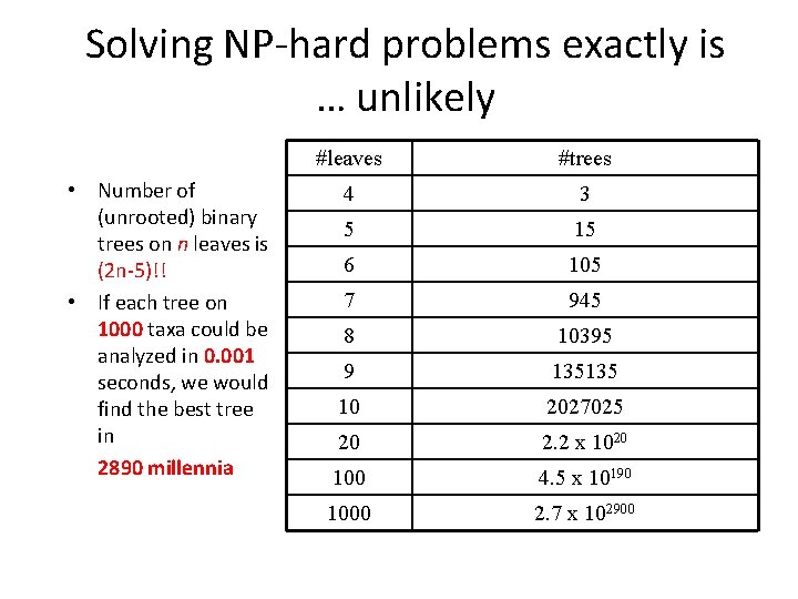
Solving NP-hard problems exactly is … unlikely • Number of (unrooted) binary trees on n leaves is (2 n-5)!! • If each tree on 1000 taxa could be analyzed in 0. 001 seconds, we would find the best tree in 2890 millennia #leaves #trees 4 3 5 15 6 105 7 945 8 10395 9 135135 10 2027025 20 2. 2 x 1020 100 4. 5 x 10190 1000 2. 7 x 102900

“Solving ML” • Technique 2: For each of the tree topologies, find the best numerical parameters (i. e. , substitution probabilities p(e) for every edge e). • Problem: Exponentially many trees on n sequences, and calculating the best setting of the parameters on any given tree is hard! Even so, there are hill-climbing heuristics for both of these calculations (finding parameter settings, and finding trees).

Maximum Likelihood • Input: sequence data S, • Output: the model tree (T, Θ) (where Θ denotes the set of substitution probabilities on each of the branches of the tree T) s. t. Pr(S|(T, Θ)) is maximized. NP-hard to find best tree. Important in practice. Good heuristics (RAx. ML, Fast. Tree, IQTree, Phy. ML, and others)

“Solving ML” • Given model tree: – Change tree topology and/or substitution probabilities – Score new model tree under likelihood (i. e. , calculate the probability of the data given the model tree) – Accept new model tree if probability goes up – Perhaps accept anyway with some small probability

“Solving ML” • Given model tree: – Change tree topology and/or substitution probabilities – Score new model tree under likelihood (i. e. , calculate the probability of the data given the model tree) – Accept new model tree if probability goes up – Perhaps accept anyway with some small probability

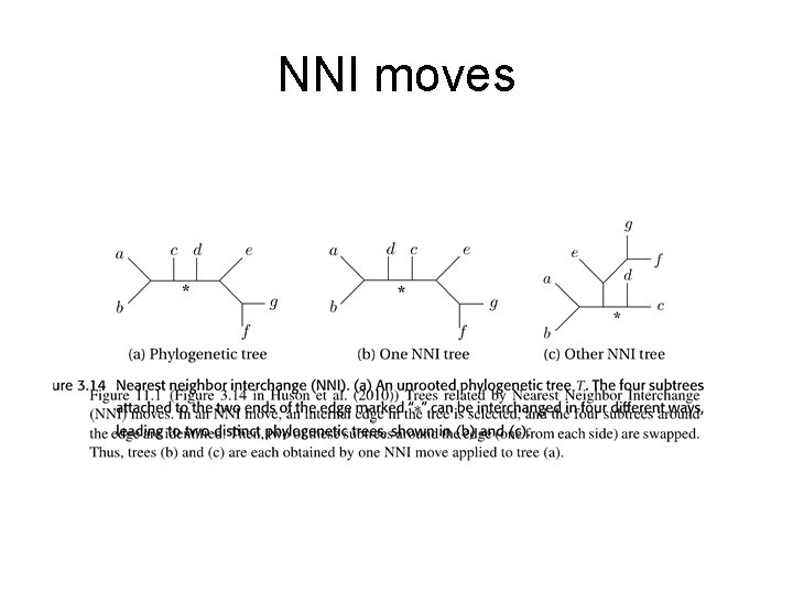
NNI moves

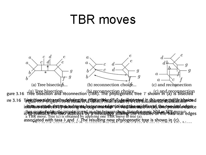
TBR moves

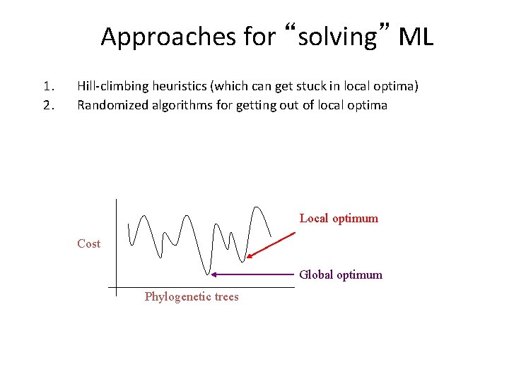
Approaches for “solving” ML 1. 2. Hill-climbing heuristics (which can get stuck in local optima) Randomized algorithms for getting out of local optima Local optimum Cost Global optimum Phylogenetic trees

“Solving ML” • Given model tree: – Change tree topology and/or substitution probabilities – Score new model tree under likelihood (i. e. , calculate the probability of the data given the model tree) – Accept new model tree if probability goes up – Perhaps accept anyway with some small probability

Calculating probability of data, given CFN model tree Basic challenge: • Given set S of binary sequences and a CFN model tree T, what is the probability that T generates S?

Computing the probability of the data • Given a model tree (with all the parameters set) and character data at the leaves, you can compute the probability of the data. • Small trees can be done by hand (brute-force technique). • Large examples are computationally intensive - but still polynomial time (using dynamic programming, similar to Sankoff’s algorithm for MP on a fixed tree).

Brute Force Technique • Assume you have the CFN model tree on n leaves (with substitution probabilities on the edges). • To calculate the probability of a sequence alignment with k sites, you can use the Brute Force technique (all ways of labelling internal nodes): – Running time is O(k 2 n). (Question: what would this be for Jukes-Cantor? ) – Not polynomial.

Computing the probability of the data • Given a model tree (with all the parameters set) and character data at the leaves, you can compute the probability of the data. • Small trees can be done by hand (brute-force technique). • Large examples are computationally intensive - but still polynomial time (using dynamic programming, similar to Sankoff’s algorithm for MP on a fixed tree).

Computing the probability of the data • Given a model tree (with all the parameters set) and character data at the leaves, you can compute the probability of the data. • Small trees can be done by hand (brute-force technique). • Large examples are computationally intensive - but still polynomial time (using Felsenstein’s Pruning Algorithm).

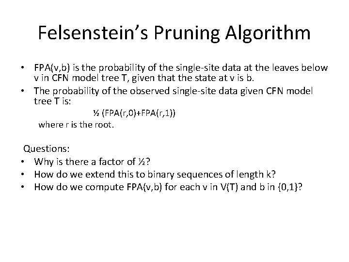
Felsenstein’s Pruning Algorithm • FPA(v, b) is the probability of the single-site data at the leaves below v in CFN model tree T, given that the state at v is b. • The probability of the observed single-site data given CFN model tree T is: ½ (FPA(r, 0)+FPA(r, 1)) where r is the root. Questions: • Why is there a factor of ½? • How do we extend this to binary sequences of length k? • How do we compute FPA(v, b) for each v in V(T) and b in {0, 1}?

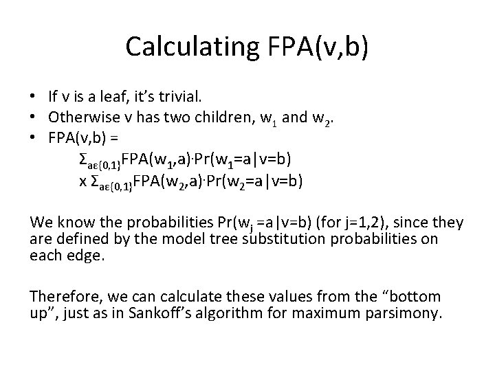
Calculating FPA(v, b) • If v is a leaf, it’s trivial. • Otherwise v has two children, w 1 and w 2. • FPA(v, b) = Σaε{0, 1}FPA(w 1, a). Pr(w 1=a|v=b) x Σaε{0, 1}FPA(w 2, a). Pr(w 2=a|v=b) We know the probabilities Pr(wj =a|v=b) (for j=1, 2), since they are defined by the model tree substitution probabilities on each edge. Therefore, we can calculate these values from the “bottom up”, just as in Sankoff’s algorithm for maximum parsimony.

Maximum Likelihood • Input: sequence data S, • Output: the model tree (T, Θ) (where Θ denotes the set of substitution probabilities on each of the branches of the tree T) s. t. Pr(S|(T, Θ)) is maximized. NP-hard to find best tree. Important in practice. Good heuristics (RAx. ML, Fast. Tree, IQTree, Phy. ML, and others)

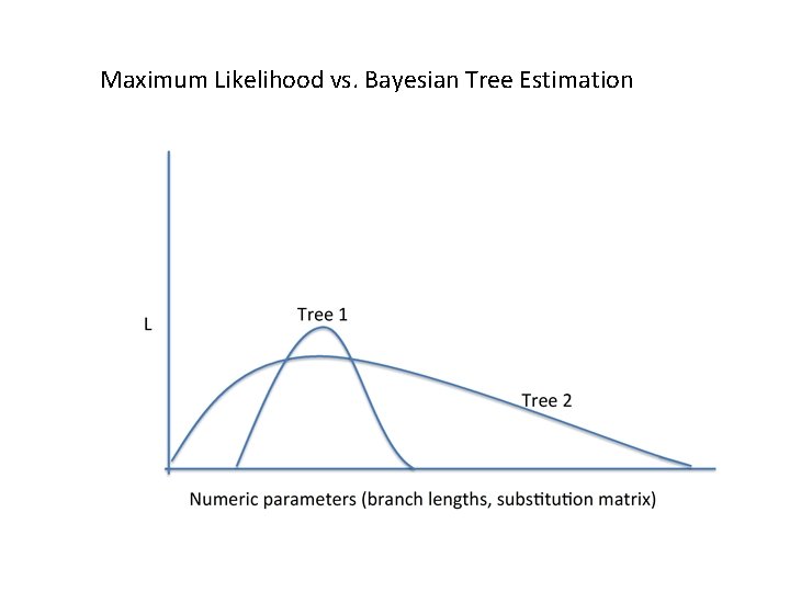
Statistical Methods • Maximum Likelihood: find model tree most likely to have generated the observed data • Bayesian Estimation: output distribution of tree topologies in proportion to their likelihood for having generated the observed data (marginalizing over all the possible numeric parameters) R (General Time Reversible) model

Statistical Methods • Maximum Likelihood: find model tree most likely to have generated the observed data • Bayesian Estimation: output distribution of tree topologies in proportion to their likelihood for having generated the observed data (marginalizing over all the possible numeric parameters) R (General Time Reversible) model

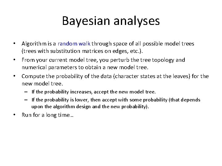
Bayesian analyses • Algorithm is a random walk through space of all possible model trees (trees with substitution matrices on edges, etc. ). • From your current model tree, you perturb the tree topology and numerical parameters to obtain a new model tree. • Compute the probability of the data (character states at the leaves) for the new model tree. – If the probability increases, accept the new model tree. – If the probability is lower, then accept with some probability (that depends upon the algorithm design and the new probability). • Run for a long time…

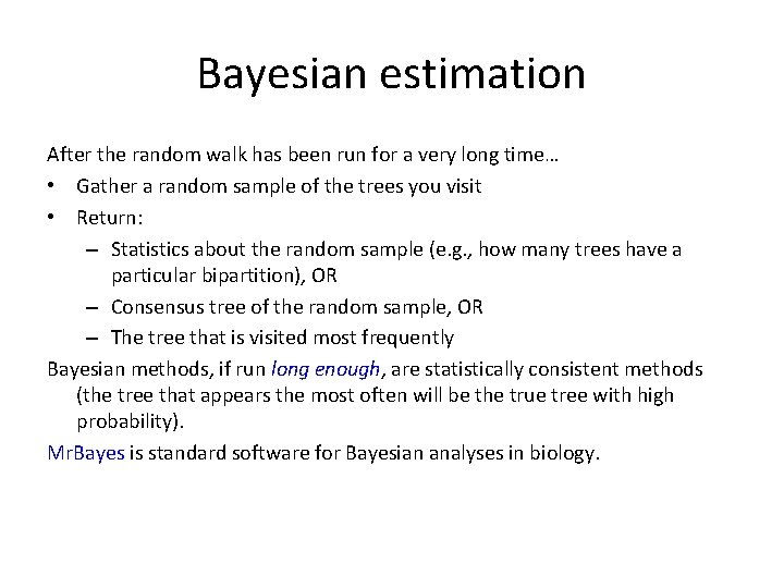
Bayesian estimation After the random walk has been run for a very long time… • Gather a random sample of the trees you visit • Return: – Statistics about the random sample (e. g. , how many trees have a particular bipartition), OR – Consensus tree of the random sample, OR – The tree that is visited most frequently Bayesian methods, if run long enough, are statistically consistent methods (the tree that appears the most often will be the true tree with high probability). Mr. Bayes is standard software for Bayesian analyses in biology.

Maximum Likelihood vs. Bayesian Tree Estimation

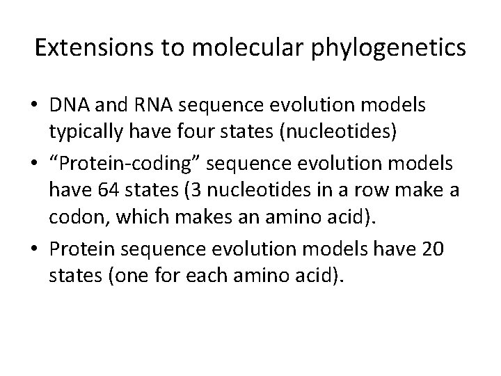
Extensions to molecular phylogenetics • DNA and RNA sequence evolution models typically have four states (nucleotides) • “Protein-coding” sequence evolution models have 64 states (3 nucleotides in a row make a codon, which makes an amino acid). • Protein sequence evolution models have 20 states (one for each amino acid).

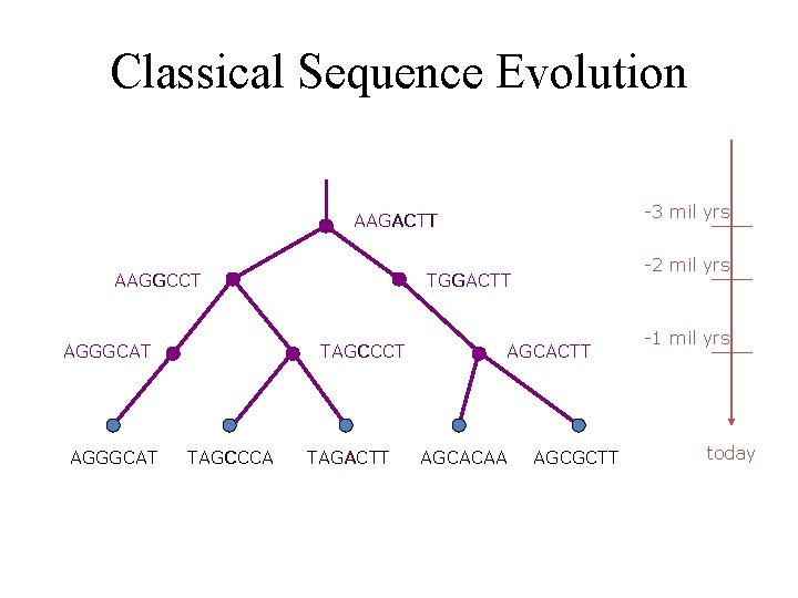
Classical Sequence Evolution -3 mil yrs AAGACTT AAGGCCT AGGGCAT TAGCCCA -2 mil yrs TGGACTT TAGACTT AGCACAA AGCGCTT -1 mil yrs today

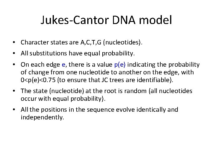
Jukes-Cantor DNA model • Character states are A, C, T, G (nucleotides). • All substitutions have equal probability. • On each edge e, there is a value p(e) indicating the probability of change from one nucleotide to another on the edge, with 0<p(e)<0. 75 (to ensure that JC trees are identifiable). • The state (nucleotide) at the root is random (all nucleotides occur with equal probability). • All the positions in the sequence evolve identically and independently.

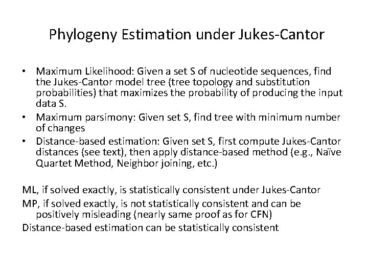
Phylogeny Estimation under Jukes-Cantor • Maximum Likelihood: Given a set S of nucleotide sequences, find the Jukes-Cantor model tree (tree topology and substitution probabilities) that maximizes the probability of producing the input data S. • Maximum parsimony: Given set S, find tree with minimum number of changes • Distance-based estimation: Given set S, first compute Jukes-Cantor distances (see text), then apply distance-based method (e. g. , Naïve Quartet Method, Neighbor joining, etc. ) ML, if solved exactly, is statistically consistent under Jukes-Cantor MP, if solved exactly, is not statistically consistent and can be positively misleading (nearly same proof as for CFN) Distance-based estimation can be statistically consistent

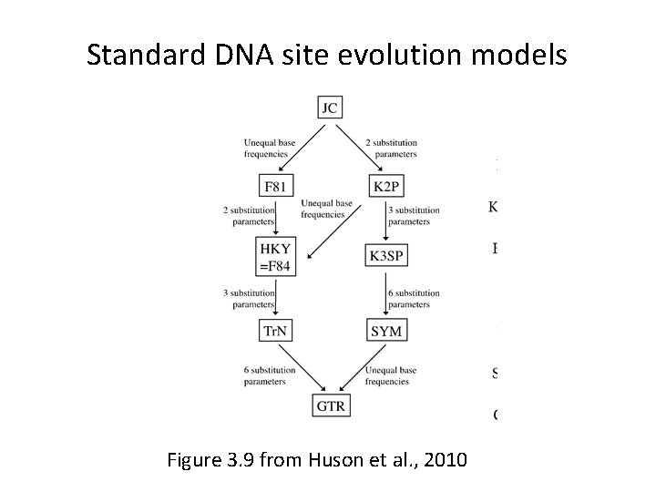
Standard DNA site evolution models Figure 3. 9 from Huson et al. , 2010

Phylogeny estimation under GTR • Generalized Time Reversible model of nucleotide sequence evolution: – Allows fairly general 4 x 4 substitution matrix – All the sites evolve i. i. d. down the tree – Most general DNA sequence evolution model used in practice (and contains all the submodels) – “logdet” distances makes distance-based estimation statistically consistent – ML still consistent, MP still inconsistent

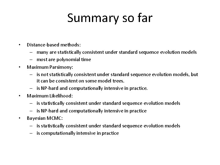
Summary so far • • Distance-based methods: – many are statistically consistent under standard sequence evolution models – most are polynomial time Maximum Parsimony: – is not statistically consistent under standard sequence evolution models, but it can be consistent on some model trees. – is NP-hard and computationally intensive in practice. Maximum Likelihood: – is statistically consistent under standard sequence evolution models – is NP-hard and computationally intensive in practice Bayesian MCMC: – is statistically consistent under standard sequence evolution models – is computationally intensive in practice

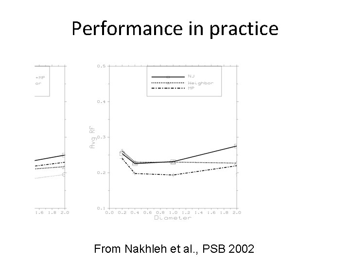
Performance on data • Statistical consistency or inconsistency is an asymptotic statement, and requires a proof; it really has nothing much to say about performance on finite data. • To evaluate performance on finite data, we use simulations. • MP is surprisingly good for many model conditions (even sometimes better than some statistically consistent methods). • Typically ML outperforms all other methods on simulated data in terms of topological accuracy.

Performance in practice From Nakhleh et al. , PSB 2002

Performance on data • Statistical consistency or inconsistency is an asymptotic statement, and requires a proof; it really has nothing much to say about performance on finite data. • To evaluate performance on finite data, we use simulations. • MP is surprisingly good for many model conditions (even sometimes better than some statistically consistent methods). • Typically ML outperforms all other methods on simulated data in terms of topological accuracy.

Current Software • RAx. ML, Fast. Tree-2, IQTree, Phy. ML, nh. Phy. ML, and others • The best ML software cannot scale to really large datasets – RAx. ML is good for long alignments if not too many sequences – Fast. Tree can analyze large datasets (even 1, 000 sequences), if alignments are short – Many datasets take weeks to analyze and use terabytes of memory • Accuracy is hard to assess on biological data, but word on the street is RAx. ML is better than Fast. Tree • RAx. ML most popular method among biologists

Research Projects • What are the conditions where Fast. Tree is less accurate than RAx. ML? • How well do methods perform when sequences evolve with heterotachy? • Can Fast. Tree be improved through simple modifications (e. g. , give it a better starting tree)?