CSCI 2950 C Lecture 8 Molecular Phylogeny Parsimony

CSCI 2950 -C Lecture 8 Molecular Phylogeny: Parsimony and Likelihood http: //cs. brown. edu/courses/csci 2950 -c/

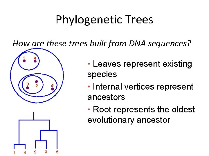
Phylogenetic Trees How are these trees built from DNA sequences? 1 4 3 1 4 5 2 2 • Leaves represent existing species • Internal vertices represent ancestors • Root represents the oldest evolutionary ancestor 3 5

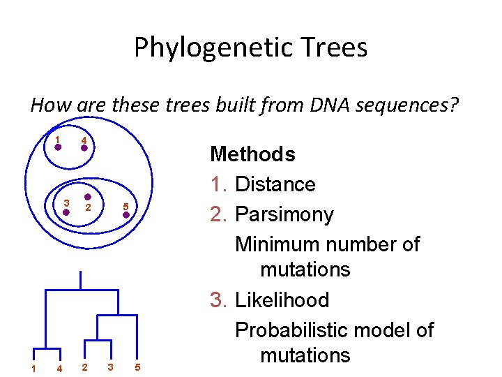
Phylogenetic Trees How are these trees built from DNA sequences? 1 4 3 1 4 5 2 2 3 5 Methods 1. Distance 2. Parsimony Minimum number of mutations 3. Likelihood Probabilistic model of mutations

Outline Last Lecture: distance-based Methods • Additive distances • 4 Point condition • UPGMA & Neighbor joining Today: • Parsimony-based methods • Sankoff + Fitch’s algorithms • Likelihood Methods • Perfect Phylogeny

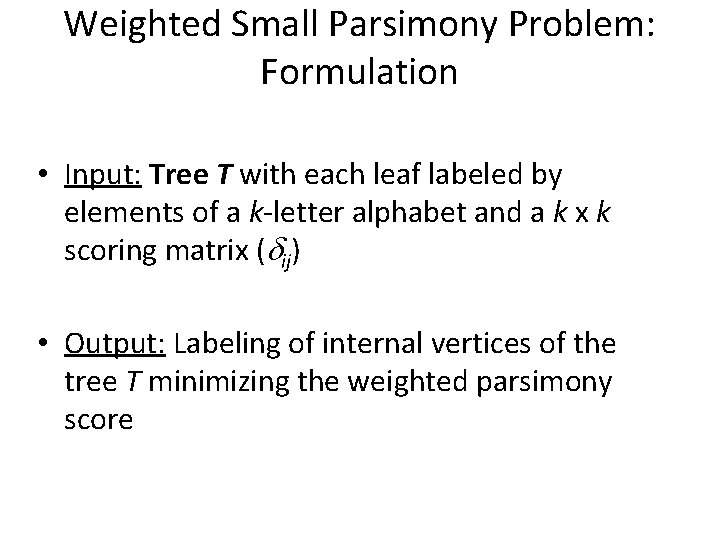
Weighted Small Parsimony Problem: Formulation • Input: Tree T with each leaf labeled by elements of a k-letter alphabet and a k x k scoring matrix ( ij) • Output: Labeling of internal vertices of the tree T minimizing the weighted parsimony score

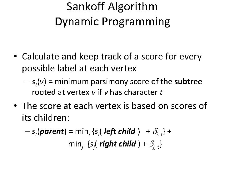
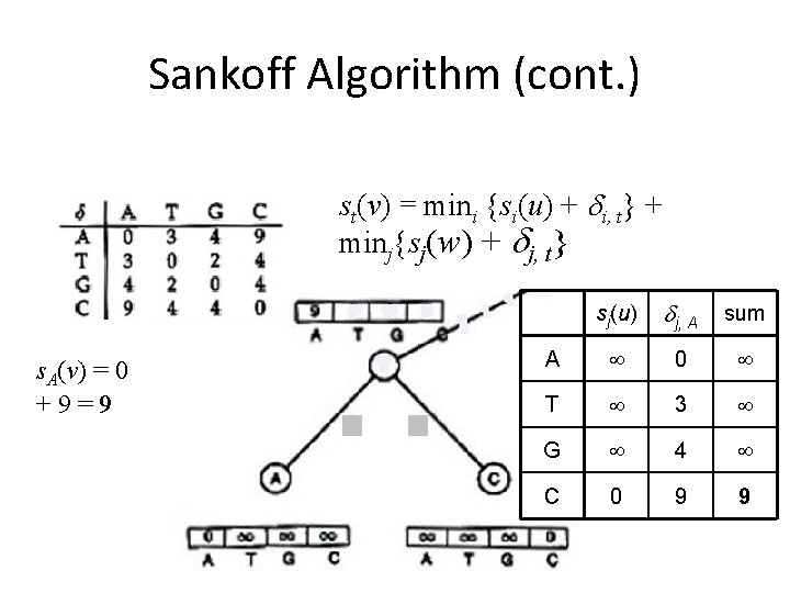
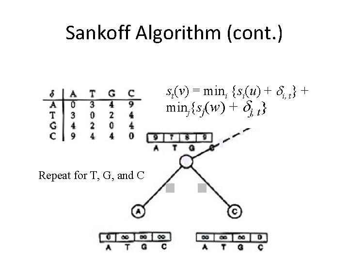
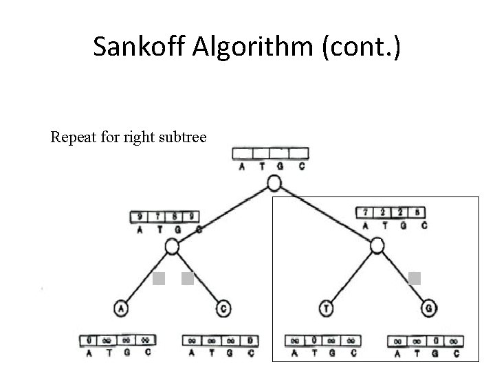
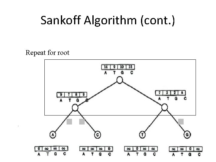
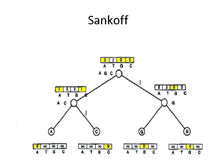
Sankoff Algorithm Dynamic Programming • Calculate and keep track of a score for every possible label at each vertex – st(v) = minimum parsimony score of the subtree rooted at vertex v if v has character t • The score at each vertex is based on scores of its children: – st(parent) = mini {si( left child ) + i, t} + minj {sj( right child ) + j, t}

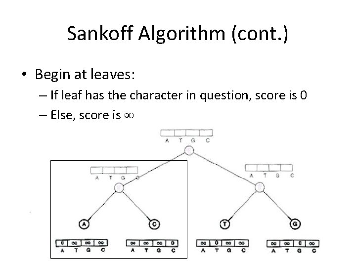
Sankoff Algorithm (cont. ) • Begin at leaves: – If leaf has the character in question, score is 0 – Else, score is

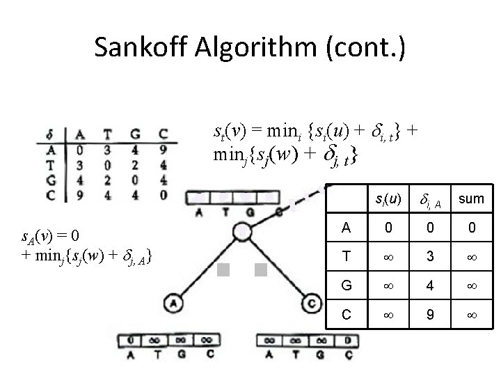
Sankoff Algorithm (cont. ) st(v) = mini {si(u) + i, t} + minj{sj(w) + j, t} s. A(v) = 0 mini{si(u) + i, A} + minj{sj(w) + j, A} si(u) i, A sum A 0 0 0 T 3 G 4 C 9

Sankoff Algorithm (cont. ) st(v) = mini {si(u) + i, t} + minj{sj(w) + j, t} s. A(v) = 0 mini{si(u) + i, A} + 9 min = 9 j{sj(w) + j, A} sj(u) j, A sum A 0 T 3 G 4 C 0 9 9

Sankoff Algorithm (cont. ) st(v) = mini {si(u) + i, t} + minj{sj(w) + j, t} Repeat for T, G, and C

Sankoff Algorithm (cont. ) Repeat for right subtree

Sankoff Algorithm (cont. ) Repeat for root

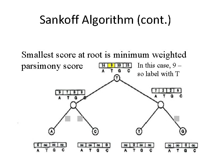
Sankoff Algorithm (cont. ) Smallest score at root is minimum weighted In this case, 9 – parsimony score so label with T

Sankoff Algorithm: Traveling down the Tree • The scores at the root vertex have been computed by going up the tree • After the scores at root vertex are computed the Sankoff algorithm moves down the tree and assign each vertex with optimal character.

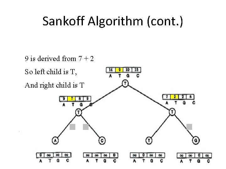
Sankoff Algorithm (cont. ) 9 is derived from 7 + 2 So left child is T, And right child is T

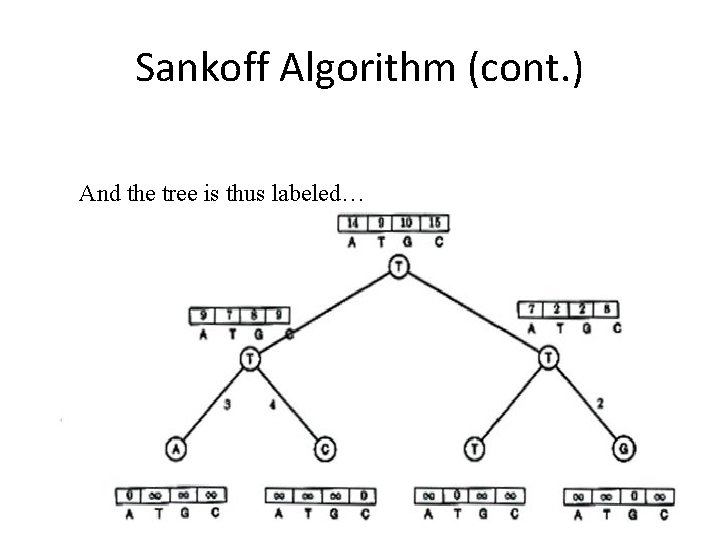
Sankoff Algorithm (cont. ) And the tree is thus labeled…

Fitch’s Algorithm • Solves Small Parsimony problem – Published 4 years before Sankoff (1971) • Assigns a set of letters to every vertex in the tree, S(v) • S(l) = observed character for each leaf l

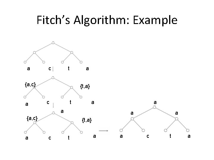
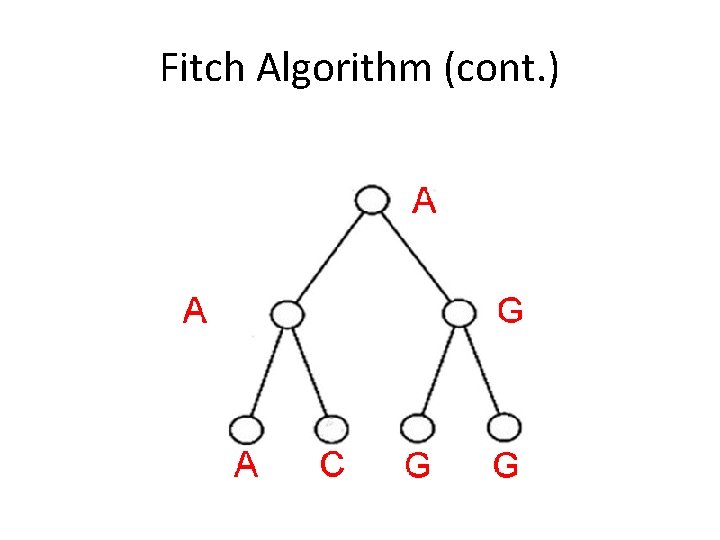
Fitch’s Algorithm: Example a c t a {a, c} a {t, a} c t a a {a, c} a a {t, a} c t a a c t a

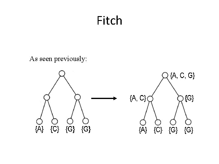
Fitch Algorithm 1) Assign a set of possible letters Sv to every vertex v, traversing the tree from leaves to root • For vertex v with children u and w: – Sv = Su “intersect” Sw if non-empty intersection Su “union” Sw , otherwise – E. g. if the node we are looking at has a left child labeled {A, C} and a right child labeled {A, T}, the node will be given the set {A, C, T}

Fitch Algorithm (cont. ) 2) Assign labels to each vertex, traversing the tree from root to leaves • Assign root arbitrarily from its set of letters • For all other vertices, if its parent’s label is in its set of letters, assign it its parent’s label • Else, choose an arbitrary letter from its set as its label

Fitch Algorithm (cont. )

Fitch vs. Sankoff • Both have an O(nk) runtime • Are they actually different? • Let’s compare …

Fitch As seen previously:

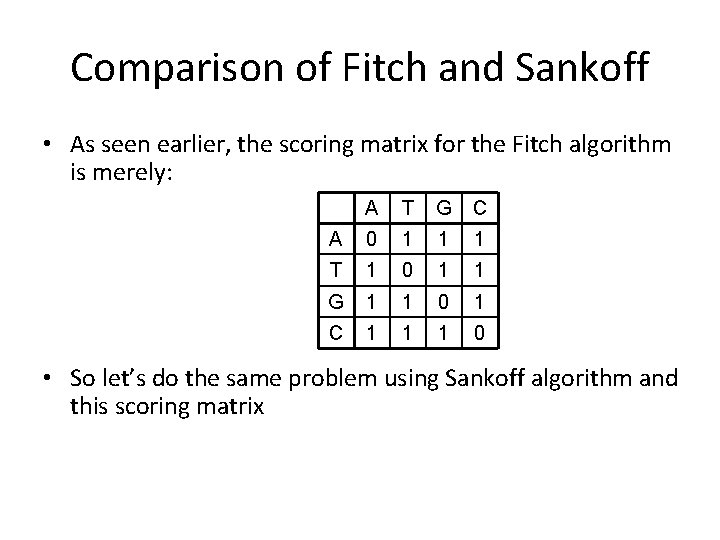
Comparison of Fitch and Sankoff • As seen earlier, the scoring matrix for the Fitch algorithm is merely: A T G C A 0 1 1 1 T 1 0 1 1 G 1 1 0 1 C 1 1 1 0 • So let’s do the same problem using Sankoff algorithm and this scoring matrix

Sankoff

Sankoff vs. Fitch • The Sankoff algorithm gives the same set of optimal labels as the Fitch algorithm • For Sankoff algorithm, character t is optimal for vertex v if st(v) = min 1<i<ksi(v) • Let Sv = set of optimal letters for v. • Then – Sv = Su “intersect” Sw if non-empty intersection Su “union” Sw , otherwise • This is also the Fitch recurrence • The two algorithms are identical

Large Parsimony Problem • Input: An n x m matrix M describing n species, each represented by an m-character string • Output: A tree T with n leaves labeled by the n rows of matrix M, and a labeling of the internal vertices such that the parsimony score is minimized over all possible trees and all possible labelings of internal vertices

Large Parsimony Problem (cont. ) • Possible search space is huge, especially as n increases – (2 n – 3)!! possible rooted trees – (2 n – 5)!! possible unrooted trees • Problem is NP-complete – Exhaustive search only possible w/ small n(< 10) • Hence, branch and bound or heuristics used

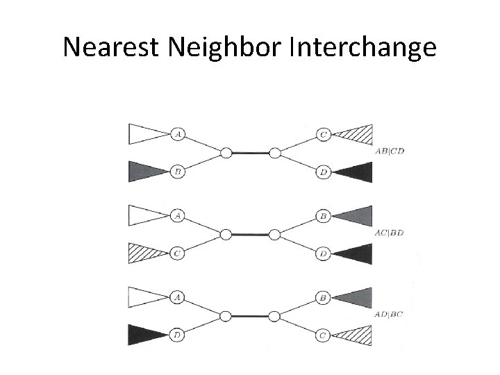
Nearest Neighbor Interchange A Greedy Algorithm • A Branch Swapping algorithm • Only evaluates a subset of all possible trees • Defines a neighbor of a tree as one reachable by a nearest neighbor interchange – A rearrangement of the four subtrees defined by one internal edge – Only three different rearrangements per edge

Nearest Neighbor Interchange

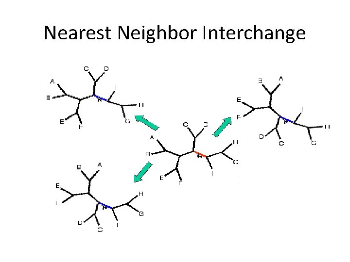
Nearest Neighbor Interchange • Start with an arbitrary tree and check its neighbors • Move to a neighbor if it provides the best improvement in parsimony score • No way of knowing if the result is the most parsimonious tree • Could be stuck in local optimum

Nearest Neighbor Interchange

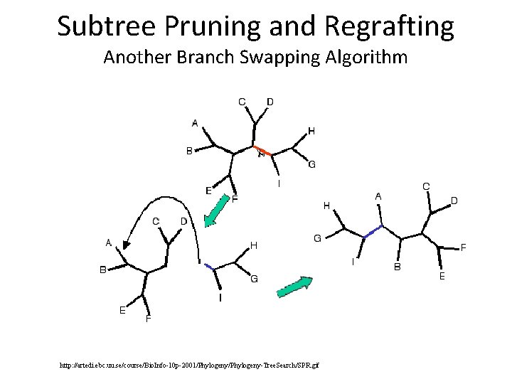
Subtree Pruning and Regrafting Another Branch Swapping Algorithm http: //artedi. ebc. uu. se/course/Bio. Info-10 p-2001/Phylogeny-Tree. Search/SPR. gif

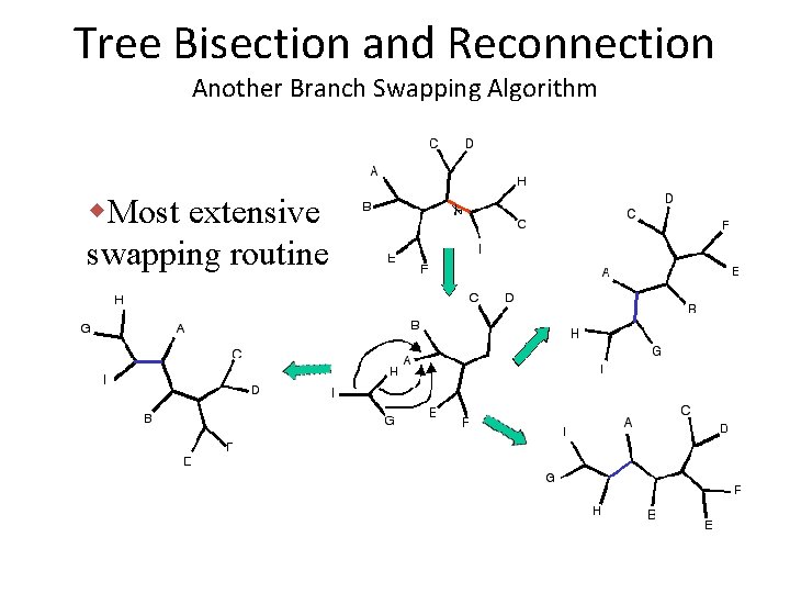
Tree Bisection and Reconnection Another Branch Swapping Algorithm w. Most extensive swapping routine

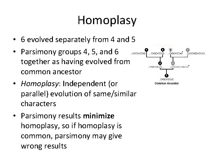
Homoplasy • Given: – – – – 1: CAGCAGCAG 2: CAGCAGCAG 3: CAGCAG 4: CAGCAGCAG 5: CAGCAGCAG 6: CAGCAGCAG 7: CAGCAG • Most would group 1, 2, 4, 5, and 6 as having evolved from a common ancestor, with a single mutation leading to the presence of 3 and 7

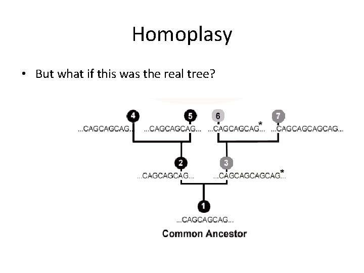
Homoplasy • But what if this was the real tree?

Homoplasy • 6 evolved separately from 4 and 5 • Parsimony groups 4, 5, and 6 together as having evolved from a common ancestor • Homoplasy: Independent (or parallel) evolution of same/similar characters • Parsimony results minimize homoplasy, so if homoplasy is common, parsimony may give wrong results

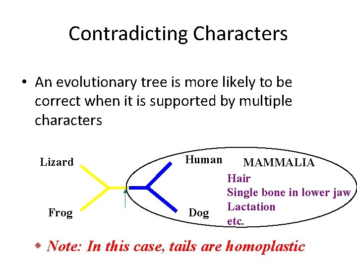
Contradicting Characters • An evolutionary tree is more likely to be correct when it is supported by multiple characters Lizard Frog Human Dog MAMMALIA Hair Single bone in lower jaw Lactation etc. w Note: In this case, tails are homoplastic

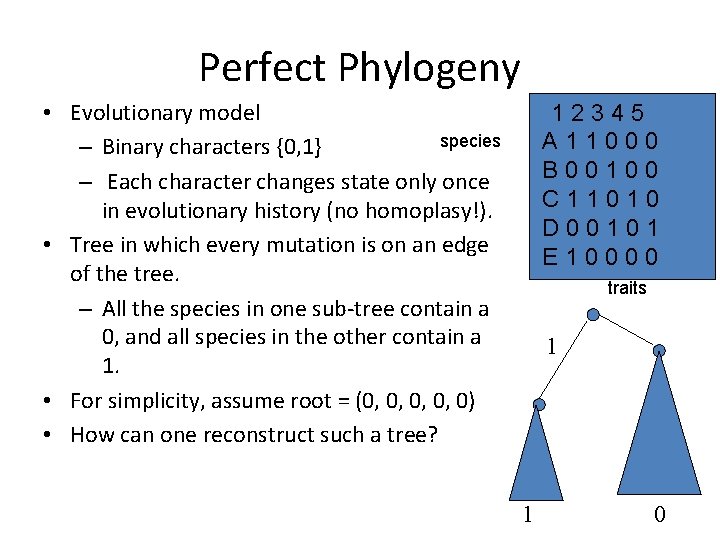
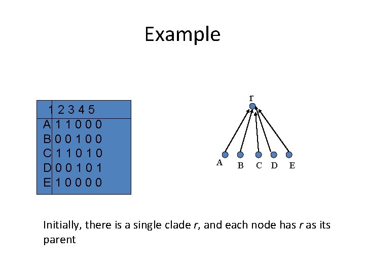
Perfect Phylogeny • Evolutionary model species – Binary characters {0, 1} – Each character changes state only once in evolutionary history (no homoplasy!). • Tree in which every mutation is on an edge of the tree. – All the species in one sub-tree contain a 0, and all species in the other contain a 1. • For simplicity, assume root = (0, 0, 0) • How can one reconstruct such a tree? 12345 A 11000 B 00100 C 11010 D 00101 E 10000 traits 1 1 0

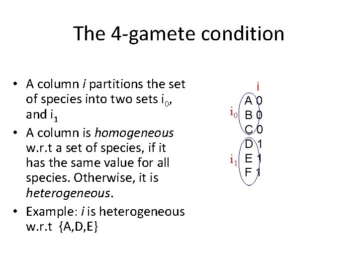
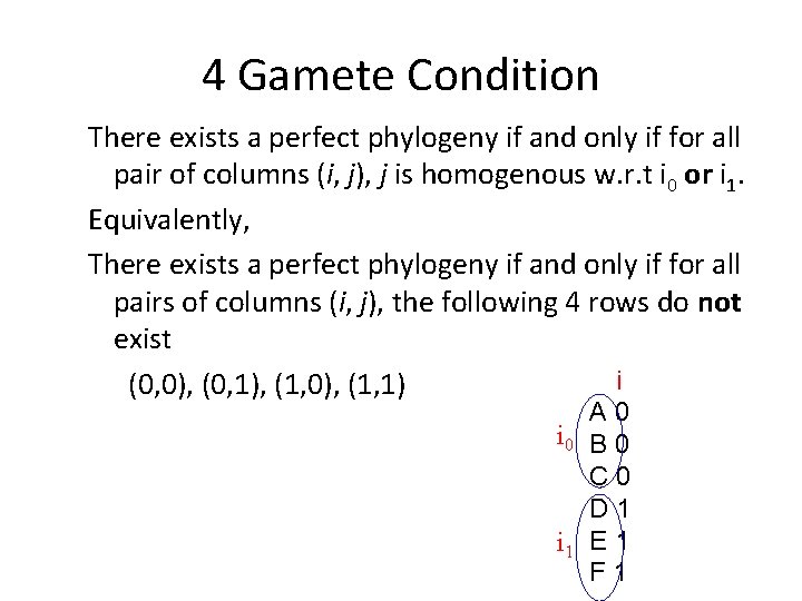
The 4 -gamete condition • A column i partitions the set of species into two sets i 0, and i 1 • A column is homogeneous w. r. t a set of species, if it has the same value for all species. Otherwise, it is heterogeneous. • Example: i is heterogeneous w. r. t {A, D, E} i A 0 i 0 B 0 C 0 D 1 i 1 E 1 F 1

4 Gamete Condition There exists a perfect phylogeny if and only if for all pair of columns (i, j), j is homogenous w. r. t i 0 or i 1. Equivalently, There exists a perfect phylogeny if and only if for all pairs of columns (i, j), the following 4 rows do not exist i (0, 0), (0, 1), (1, 0), (1, 1) A 0 i 0 B 0 C 0 D 1 i 1 E 1 F 1

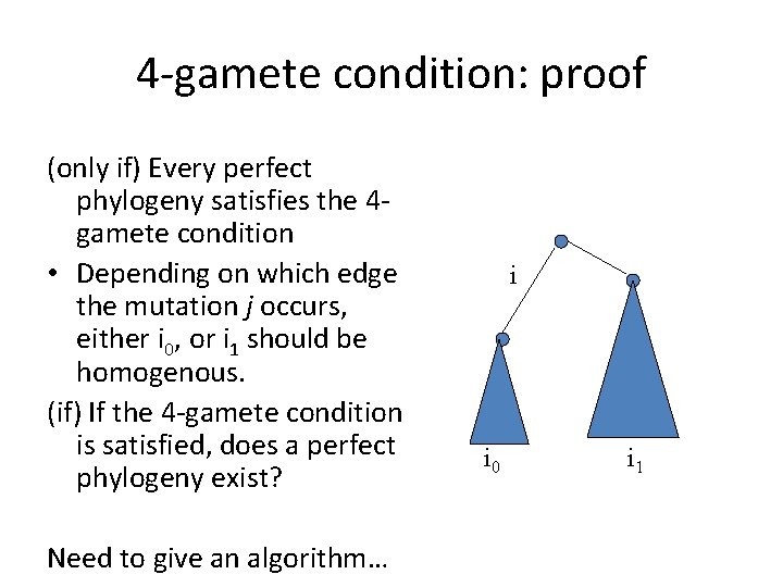
4 -gamete condition: proof (only if) Every perfect phylogeny satisfies the 4 gamete condition • Depending on which edge the mutation j occurs, either i 0, or i 1 should be homogenous. (if) If the 4 -gamete condition is satisfied, does a perfect phylogeny exist? Need to give an algorithm… i i 0 i 1

An algorithm for constructing a perfect phylogeny • We will consider the case where 0 is the ancestral state, and 1 is the mutated state. This will be fixed later. • In any tree, each node (except the root) has a single parent. – It is sufficient to construct a parent for every node. • In each step, we add a column and refine some of the nodes containing multiple children. • Stop if all columns have been considered.

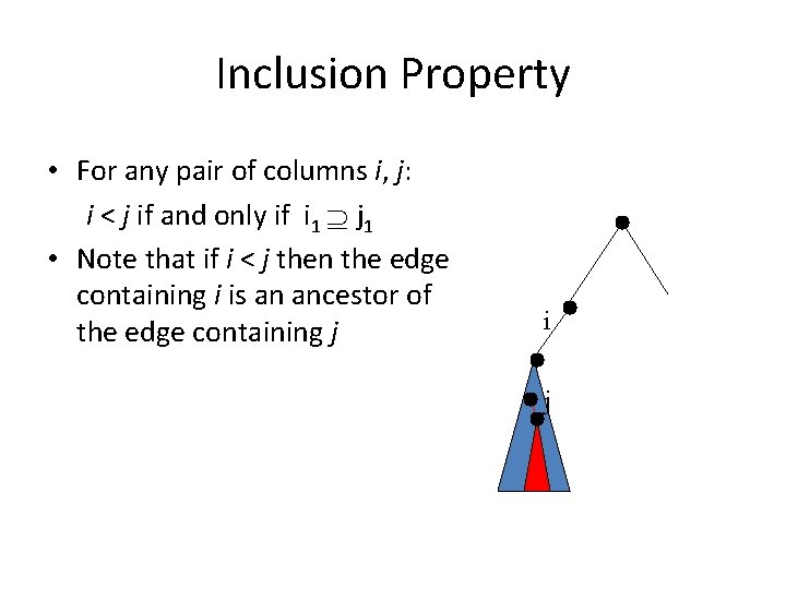
Inclusion Property • For any pair of columns i, j: i < j if and only if i 1 j 1 • Note that if i < j then the edge containing i is an ancestor of the edge containing j i j

Example 12345 A 11000 B 00100 C 11010 D 00101 E 10000 r A B C D E Initially, there is a single clade r, and each node has r as its parent

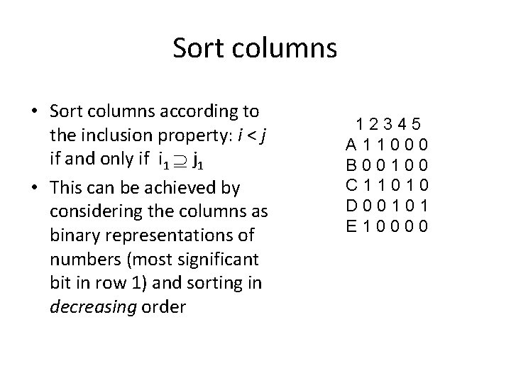
Sort columns • Sort columns according to the inclusion property: i < j if and only if i 1 j 1 • This can be achieved by considering the columns as binary representations of numbers (most significant bit in row 1) and sorting in decreasing order 12345 A 11000 B 00100 C 11010 D 00101 E 10000

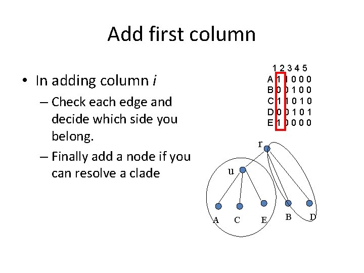
Add first column 12345 A 11000 B 00100 C 11010 D 00101 E 10000 • In adding column i – Check each edge and decide which side you belong. – Finally add a node if you can resolve a clade r u A C E B D

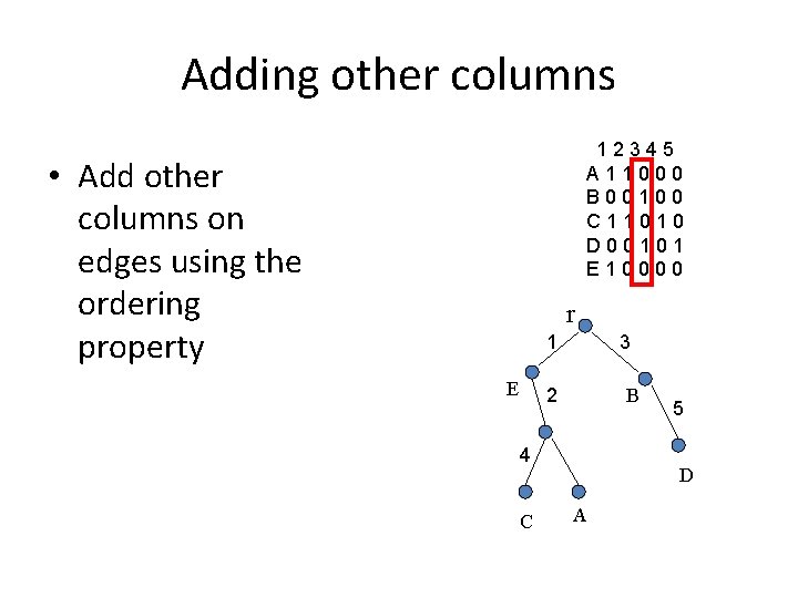
Adding other columns 12345 A 11000 B 00100 C 11010 D 00101 E 10000 • Add other columns on edges using the ordering property r 1 E 3 2 B 4 C 5 D A

Unrooted case • Switch the values in each column, so that 0 is the majority element. • Apply the algorithm for the rooted case

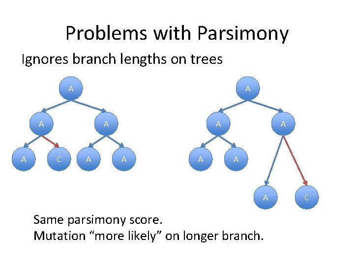
Problems with Parsimony Ignores branch lengths on trees A A A C A A A A Same parsimony score. Mutation “more likely” on longer branch. C

Maximum Likelihood See Class Notes

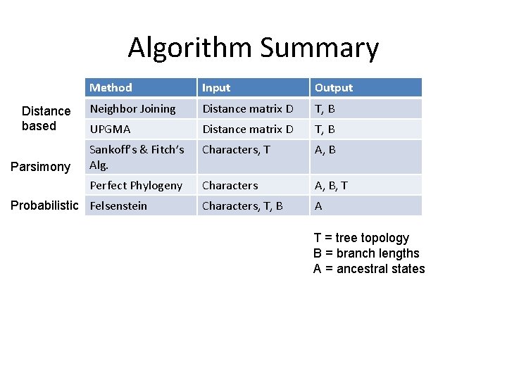
Algorithm Summary Distance based Parsimony Method Input Output Neighbor Joining Distance matrix D T, B UPGMA Distance matrix D T, B Sankoff’s & Fitch’s Alg. Characters, T A, B Perfect Phylogeny Characters A, B, T Characters, T, B A Probabilistic Felsenstein T = tree topology B = branch lengths A = ancestral states

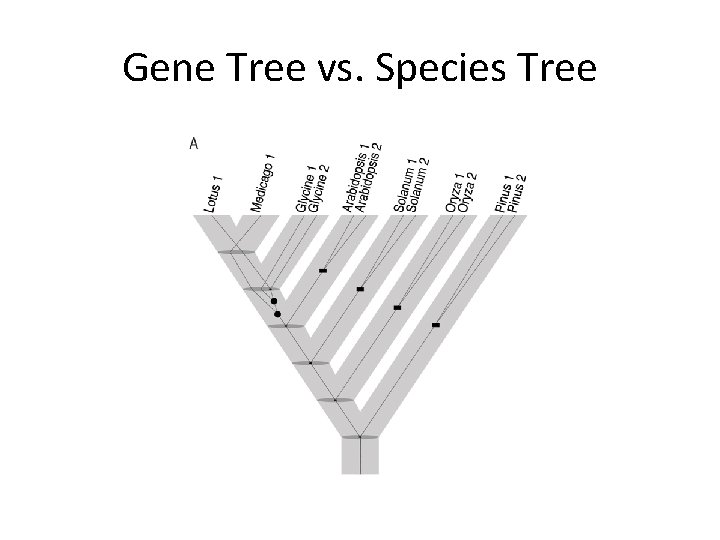
Gene Tree vs. Species Tree

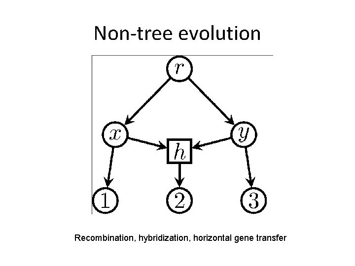
Non-tree evolution Recombination, hybridization, horizontal gene transfer

Using Multiple Methods • Important to keep in mind that reliance on purely one method for phylogenetic analysis provides incomplete picture • When different methods (parsimony, distance -based, etc. ) all give same result, more likely that the result is correct

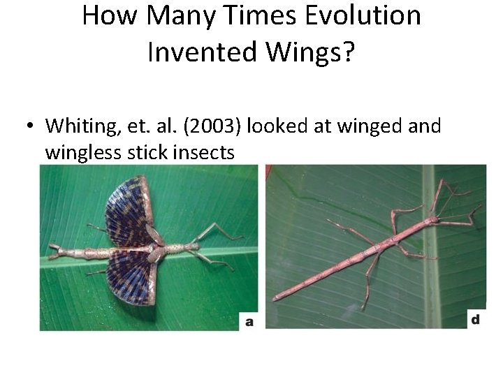
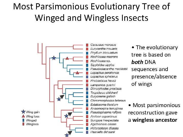
How Many Times Evolution Invented Wings? • Whiting, et. al. (2003) looked at winged and wingless stick insects

Reinventing Wings • Previous studies had shown winged wingless transitions • Wingless winged transition much more complicated (need to develop many new biochemical pathways) • Used multiple tree reconstruction techniques, all of which required reevolution of wings

Most Parsimonious Evolutionary Tree of Winged and Wingless Insects • The evolutionary tree is based on both DNA sequences and presence/absence of wings • Most parsimonious reconstruction gave a wingless ancestor

Will Wingless Insects Fly Again? • Since the most parsimonious reconstructions all required the re-invention of wings, it is most likely that wing developmental pathways are conserved in wingless stick insects

Phylogenetic Analysis of HIV Virus • Lafayette, Louisiana, 1994 – A woman claimed her ex-lover (who was a physician) injected her with HIV+ blood • Records show the physician had drawn blood from an HIV+ patient that day • But how to prove the blood from that HIV+ patient ended up in the woman?

HIV Transmission • HIV has a high mutation rate, which can be used to trace paths of transmission • Two people who got the virus from two different people will have very different HIV sequences • Three different tree reconstruction methods (including parsimony) were used to track changes in two genes in HIV (gp 120 and RT)

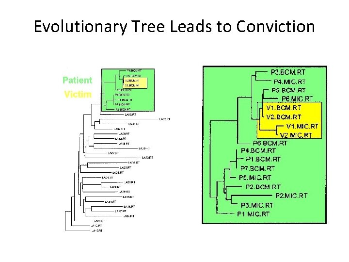
HIV Transmission • Took multiple samples from the patient, the woman, and controls (non-related HIV+ people) • In every reconstruction, the woman’s sequences were found to be evolved from the patient’s sequences, indicating a close relationship between the two • Nesting of the victim’s sequences within the patient sequence indicated the direction of transmission was from patient to victim • This was the first time phylogenetic analysis was used in a court case as evidence (Metzker, et. al. , 2002)

Evolutionary Tree Leads to Conviction

Current popular methods HUNDREDS of programs available! http: //evolution. genetics. washington. edu/phylip/software. html#methods Some recommended programs: • Discrete—Parsimony-based – Rec-1 -DCM 3 http: //www. cs. utexas. edu/users/tandy/mp. html Tandy Warnow and colleagues • Probabilistic – SEMPHY http: //www. cs. huji. ac. il/labs/compbio/semphy/ Nir Friedman and colleagues

Sources • Metzker et al. Molecular evidence of HIV-1 transmission in a criminal case. PNAS 2002. • Whiting et al. “Loss and recovery of wings in stick insects” Nature 421, 264 -267 • Serafim Batzoglou http: //ai. stanford. edu/~serafim/CS 262_2006/ (Phylogeny slides) • http: //bioalgorithms. info (Phylogeny slides) • V. Bafna (Perfect Phylogeny slides)