TIPP and SEPP plus PASTA Tandy Warnow Department

TIPP and SEPP (plus PASTA) Tandy Warnow Department of Computer Science The University of Illinois at Urbana-Champaign

TIPP https: //github. com/smirarab/sepp TIPP (Bioinformatics 2014) performs marker-gene based: • taxonomic identification (what is this read? ) and • metagenomic abundance profiling (at some taxonomic level) TIPP uses PASTA (J. Comp. Biol. 2015) to compute large-scale multiple sequence alignments and phylogenetic trees, and SEPP (Pacific Symposium on Biocomputing 2012) to add short reads into taxonomies (more generally, “phylogenetic placement”) TIPP and SEPP each use an “ensemble of profile Hidden Markov Models” (e. HMMs) to obtain high accuracy

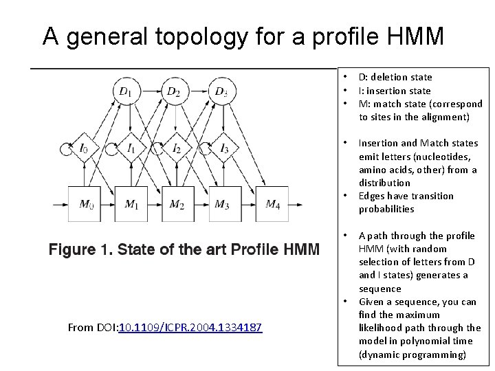
A general topology for a profile HMM • • • D: deletion state I: insertion state M: match state (correspond to sites in the alignment) • Insertion and Match states emit letters (nucleotides, amino acids, other) from a distribution Edges have transition probabilities • • • From DOI: 10. 1109/ICPR. 2004. 1334187 A path through the profile HMM (with random selection of letters from D and I states) generates a sequence Given a sequence, you can find the maximum likelihood path through the model in polynomial time (dynamic programming)

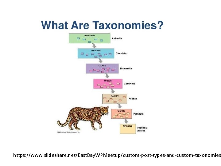
https: //www. slideshare. net/East. Bay. WPMeetup/custom-post-types-and-custom-taxonomies

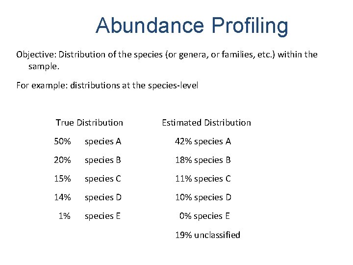
Abundance Profiling Objective: Distribution of the species (or genera, or families, etc. ) within the sample. For example: distributions at the species-level True Distribution Estimated Distribution 50% species A 42% species A 20% species B 18% species B 15% species C 11% species C 14% species D 10% species D 1% species E 0% species E 19% unclassified

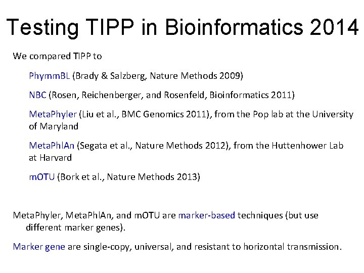
Testing TIPP in Bioinformatics 2014 We compared TIPP to Phymm. BL (Brady & Salzberg, Nature Methods 2009) NBC (Rosen, Reichenberger, and Rosenfeld, Bioinformatics 2011) Meta. Phyler (Liu et al. , BMC Genomics 2011), from the Pop lab at the University of Maryland Meta. Phl. An (Segata et al. , Nature Methods 2012), from the Huttenhower Lab at Harvard m. OTU (Bork et al. , Nature Methods 2013) Meta. Phyler, Meta. Phl. An, and m. OTU are marker-based techniques (but use different marker genes). Marker gene are single-copy, universal, and resistant to horizontal transmission.

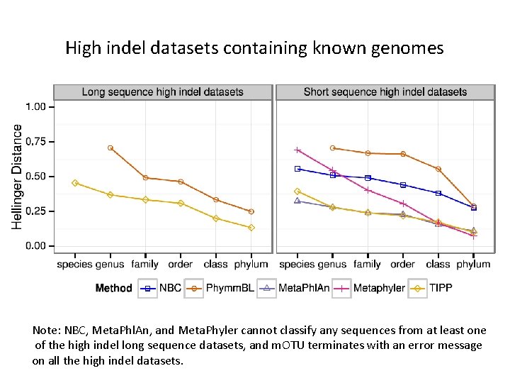
High indel datasets containing known genomes Note: NBC, Meta. Phl. An, and Meta. Phyler cannot classify any sequences from at least one of the high indel long sequence datasets, and m. OTU terminates with an error message on all the high indel datasets.

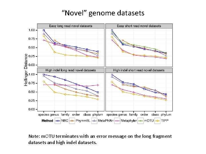
“Novel” genome datasets Note: m. OTU terminates with an error message on the long fragment datasets and high indel datasets.

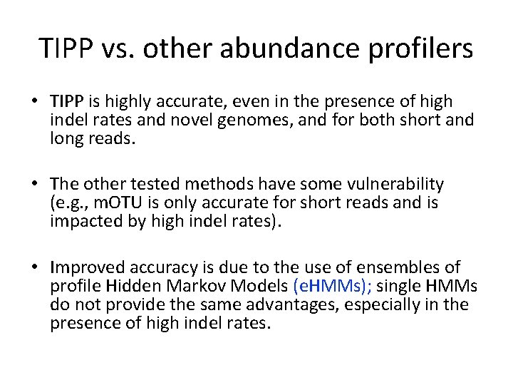
TIPP vs. other abundance profilers • TIPP is highly accurate, even in the presence of high indel rates and novel genomes, and for both short and long reads. • The other tested methods have some vulnerability (e. g. , m. OTU is only accurate for short reads and is impacted by high indel rates). • Improved accuracy is due to the use of ensembles of profile Hidden Markov Models (e. HMMs); single HMMs do not provide the same advantages, especially in the presence of high indel rates.

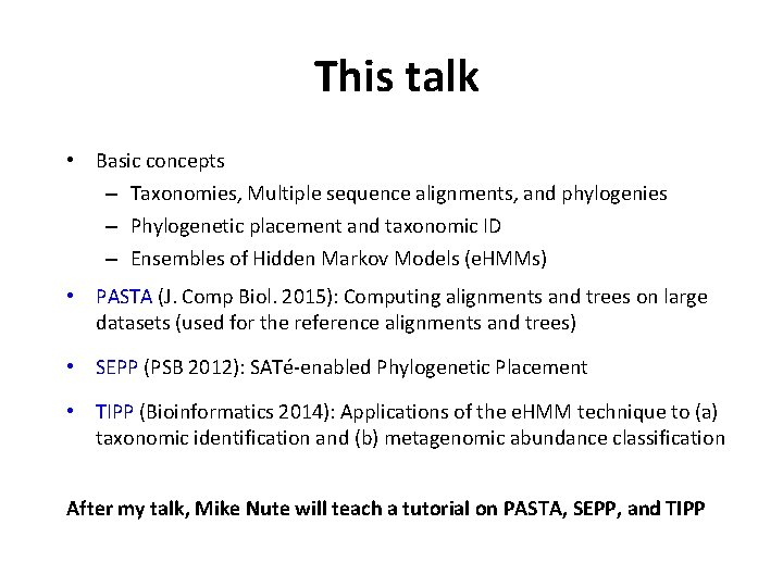
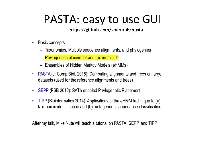
This talk • Basic concepts – Taxonomies, Multiple sequence alignments, and phylogenies – Phylogenetic placement and taxonomic ID – Ensembles of Hidden Markov Models (e. HMMs) • PASTA (J. Comp Biol. 2015): Computing alignments and trees on large datasets (used for the reference alignments and trees) • SEPP (PSB 2012): SATé-enabled Phylogenetic Placement • TIPP (Bioinformatics 2014): Applications of the e. HMM technique to (a) taxonomic identification and (b) metagenomic abundance classification After my talk, Mike Nute will teach a tutorial on PASTA, SEPP, and TIPP

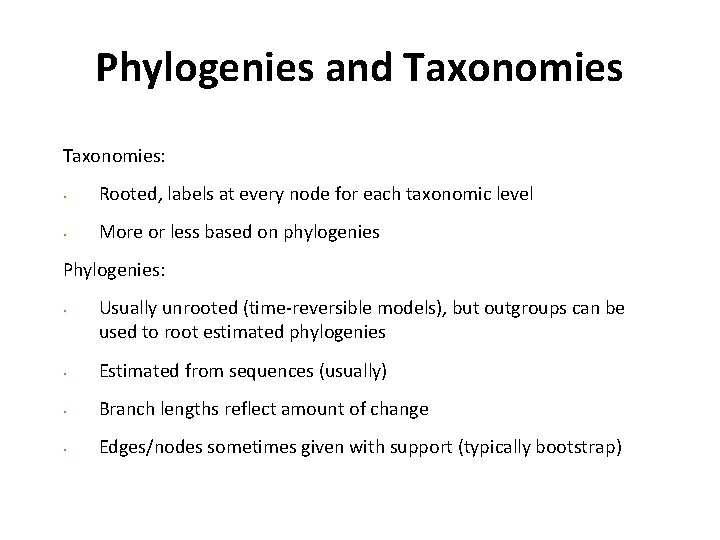
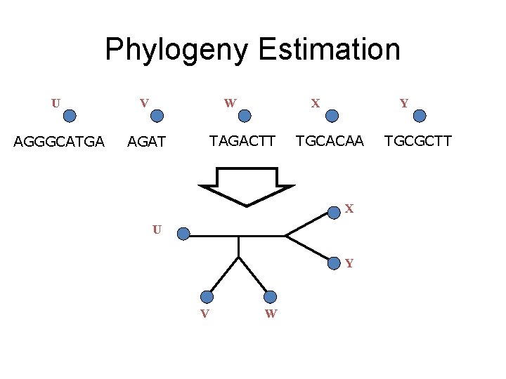
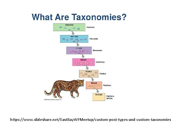
Phylogenies and Taxonomies: • Rooted, labels at every node for each taxonomic level • More or less based on phylogenies Phylogenies: • Usually unrooted (time-reversible models), but outgroups can be used to root estimated phylogenies • Estimated from sequences (usually) • Branch lengths reflect amount of change • Edges/nodes sometimes given with support (typically bootstrap)

Phylogeny Estimation U V W AGGGCATGA AGAT X TAGACTT Y TGCACAA X U Y V W TGCGCTT

Rooted neighbor-joining 16 S r. RNA phylogenetic tree of uncultured bacteria https: //www. researchgate. net/Rooted-neighbor-joining-16 S-r. RNA-gene-based-phylogenetic-tree-of-uncultured-bacteria-The_fig 1_279565247 [accessed 26 Jul, 2018]

https: //www. slideshare. net/East. Bay. WPMeetup/custom-post-types-and-custom-taxonomies

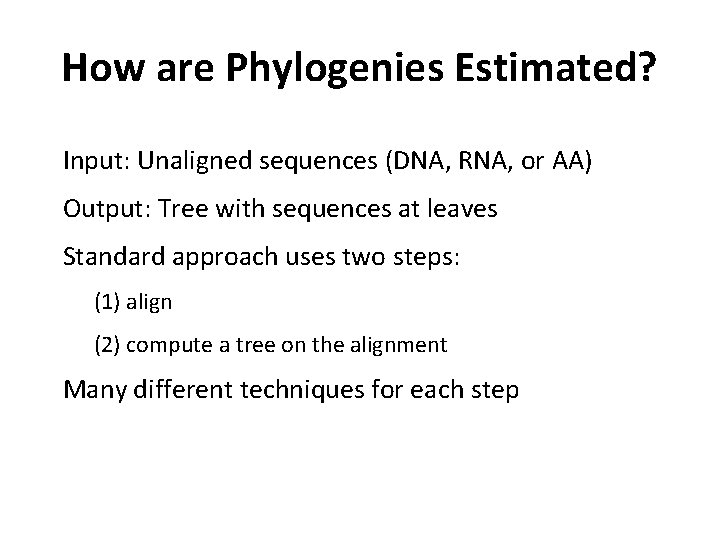
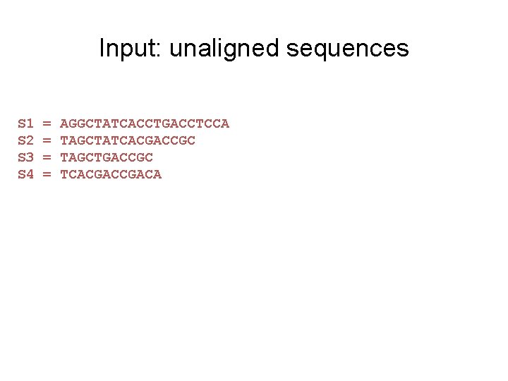
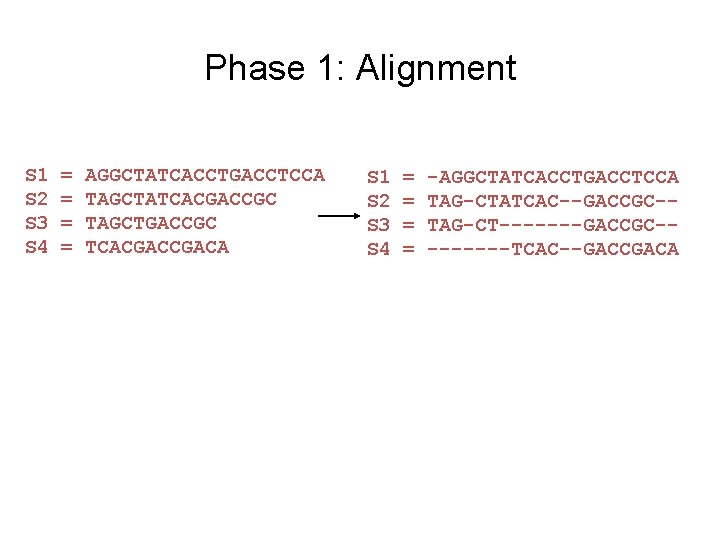
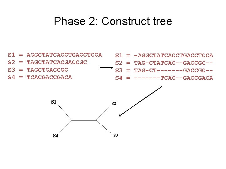
How are Phylogenies Estimated? Input: Unaligned sequences (DNA, RNA, or AA) Output: Tree with sequences at leaves Standard approach uses two steps: (1) align (2) compute a tree on the alignment Many different techniques for each step

Input: unaligned sequences S 1 S 2 S 3 S 4 = = AGGCTATCACCTGACCTCCA TAGCTATCACGACCGC TAGCTGACCGC TCACGACA

Phase 1: Alignment S 1 S 2 S 3 S 4 = = AGGCTATCACCTGACCTCCA TAGCTATCACGACCGC TAGCTGACCGC TCACGACA S 1 S 2 S 3 S 4 = = -AGGCTATCACCTGACCTCCA TAG-CTATCAC--GACCGC-TAG-CT-------GACCGC----TCAC--GACCGACA

Phase 2: Construct tree S 1 S 2 S 3 S 4 = = AGGCTATCACCTGACCTCCA TAGCTATCACGACCGC TAGCTGACCGC TCACGACA S 1 S 4 S 1 S 2 S 3 S 4 S 2 S 3 = = -AGGCTATCACCTGACCTCCA TAG-CTATCAC--GACCGC-TAG-CT-------GACCGC----TCAC--GACCGACA

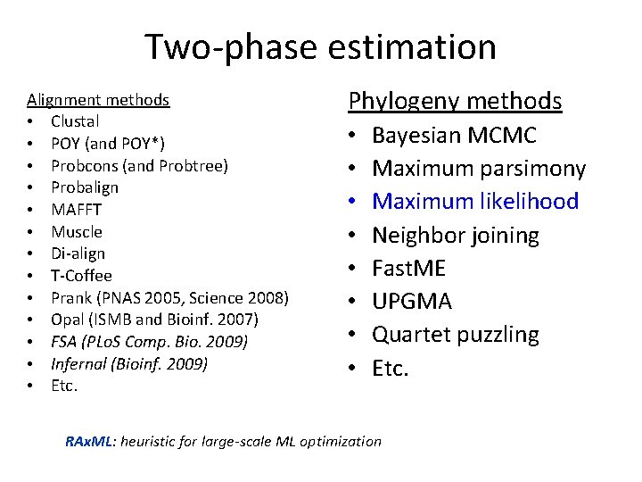
Two-phase estimation Alignment methods • Clustal • POY (and POY*) • Probcons (and Probtree) • Probalign • MAFFT • Muscle • Di-align • T-Coffee • Prank (PNAS 2005, Science 2008) • Opal (ISMB and Bioinf. 2007) • FSA (PLo. S Comp. Bio. 2009) • Infernal (Bioinf. 2009) • Etc. Phylogeny methods • • Bayesian MCMC Maximum parsimony Maximum likelihood Neighbor joining Fast. ME UPGMA Quartet puzzling Etc. RAx. ML: heuristic for large-scale ML optimization

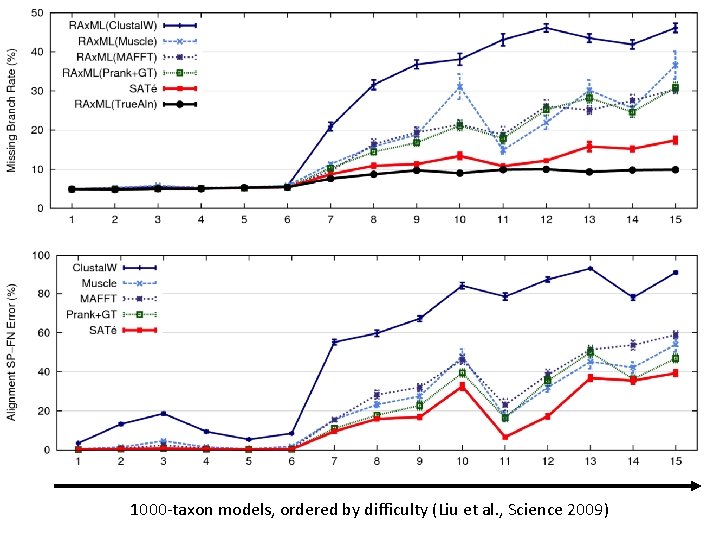
1000 -taxon models, ordered by difficulty (Liu et al. , Science 2009)

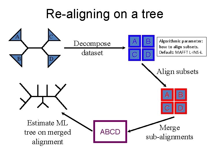
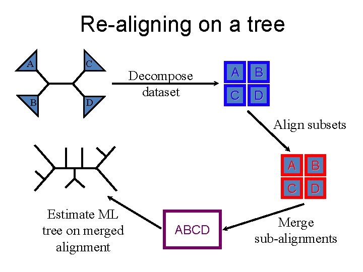
Re-aligning on a tree A B C D Decompose dataset A B C D Align subsets Estimate ML tree on merged alignment ABCD A B C D Merge sub-alignments

Re-aligning on a tree A B C D Decompose dataset A B C D Algorithmic parameter: how to align subsets. Default: MAFFT L-INS-i. Align subsets Estimate ML tree on merged alignment ABCD A B C D Merge sub-alignments

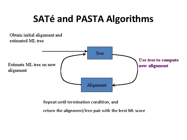
SATé and PASTA Algorithms Obtain initial alignment and estimated ML tree Tree Use tree to compute new alignment Estimate ML tree on new alignment Alignment Repeat until termination condition, and return the alignment/tree pair with the best ML score

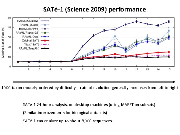
SATé-1 (Science 2009) performance 1000 -taxon models, ordered by difficulty – rate of evolution generally increases from left to right SATé-1 24 -hour analysis, on desktop machines (using MAFFT on subsets) (Similar improvements for biological datasets) SATé-1 can analyze up to about 8, 000 sequences.

SATé-1 and SATé-2 (Systematic Biology, 2012) SATé-1: up to 8 K SATé-2: up to ~50 K 1000 -taxon models ranked by difficulty

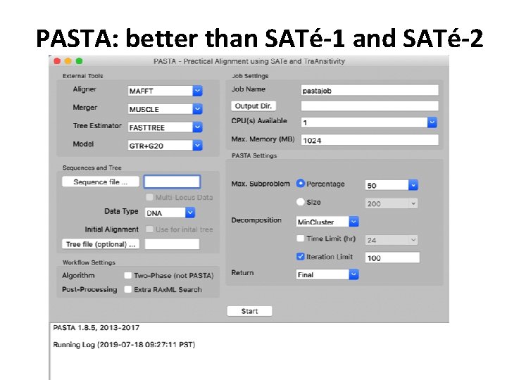
PASTA: better than SATé-1 and SATé-2

SATé and PASTA Algorithms Obtain initial alignment and estimated ML tree Tree Use tree to compute new alignment Estimate ML tree on new alignment Alignment Repeat until termination condition, and return the alignment/tree pair with the best ML score

Re-aligning on a tree A B C D Decompose dataset A B C D Align subsets Estimate ML tree on merged alignment ABCD A B C D Merge sub-alignments

PASTA: easy to use GUI https: //github. com/smirarab/pasta

The Tutorial (by Mike Nute) • PASTA for large-scale MSA and tree estimation • SEPP for taxon ID – Will show you how to run SEPP – Will show you how to use branch lengths in SEPP’s placement of reads to get interesting insights • TIPP for taxon ID and abundance profiling

This talk

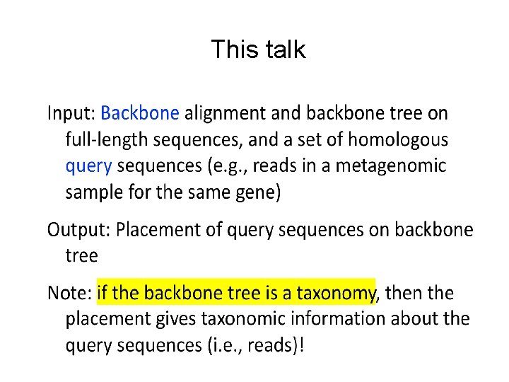
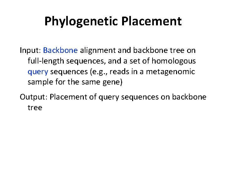
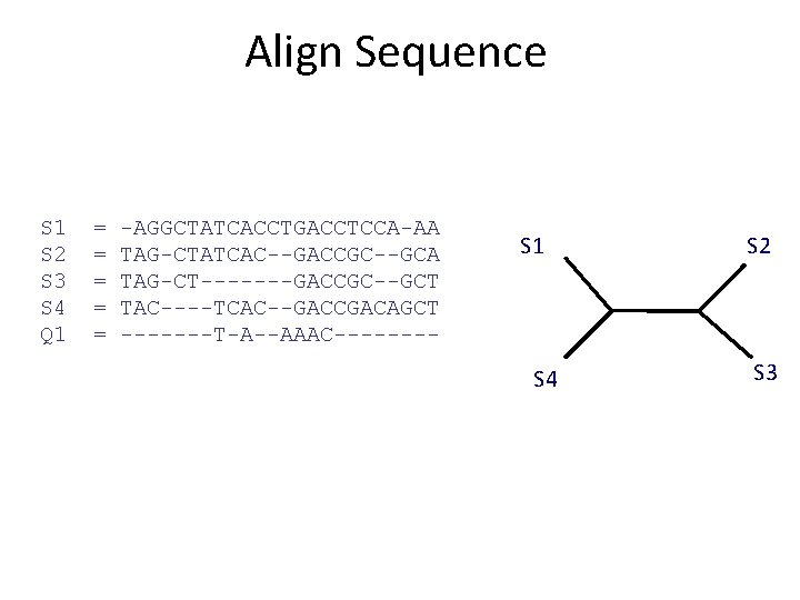
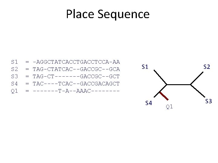
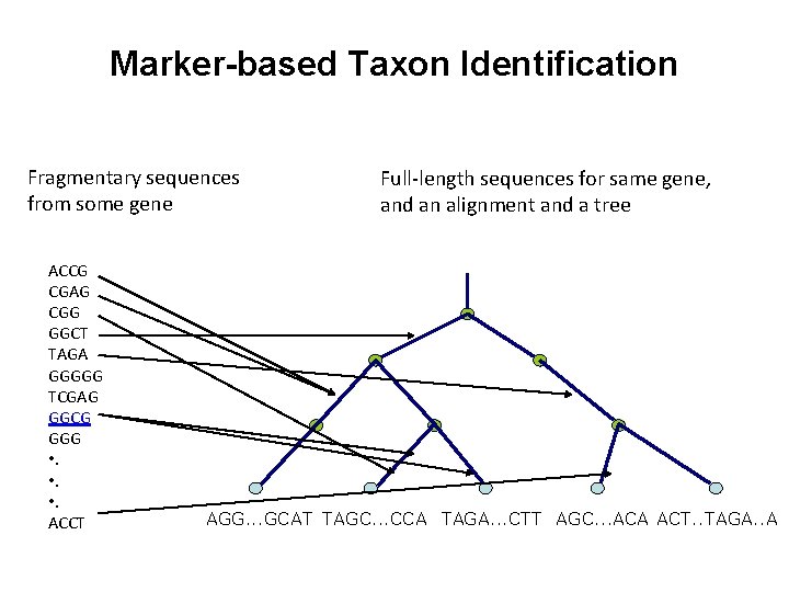
Phylogenetic Placement Input: Backbone alignment and backbone tree on full-length sequences, and a set of homologous query sequences (e. g. , reads in a metagenomic sample for the same gene) Output: Placement of query sequences on backbone tree Note: if the backbone tree is a Taxonomy, then the placement gives taxonomic information about the query sequences (i. e. , reads)!

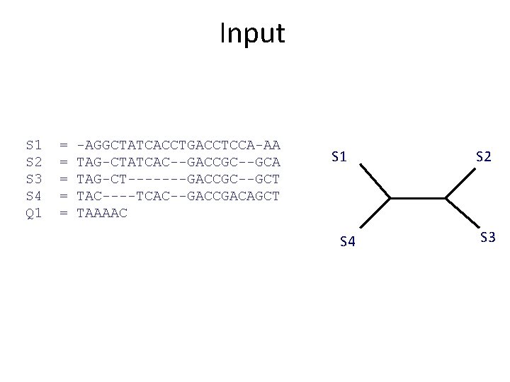
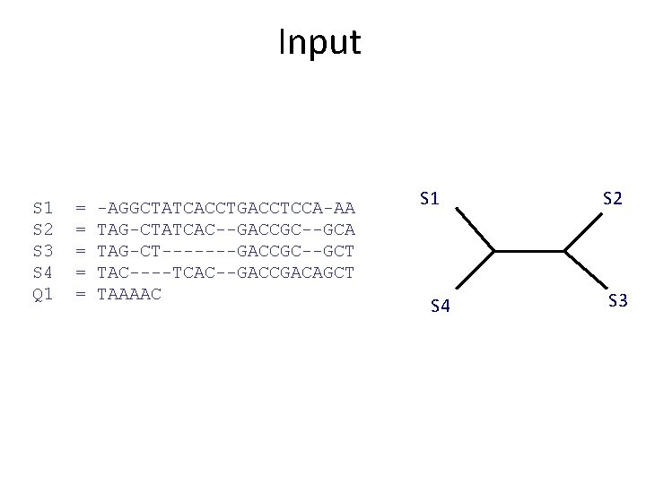
Input S 1 S 2 S 3 S 4 Q 1 = = = -AGGCTATCACCTGACCTCCA-AA TAG-CTATCAC--GACCGC--GCA TAG-CT-------GACCGC--GCT TAC----TCAC--GACCGACAGCT TAAAAC S 1 S 4 S 2 S 3

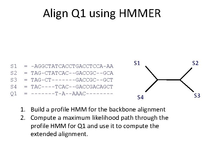
Align Sequence S 1 S 2 S 3 S 4 Q 1 = = = -AGGCTATCACCTGACCTCCA-AA TAG-CTATCAC--GACCGC--GCA TAG-CT-------GACCGC--GCT TAC----TCAC--GACCGACAGCT -------T-A--AAAC---- S 1 S 4 S 2 S 3

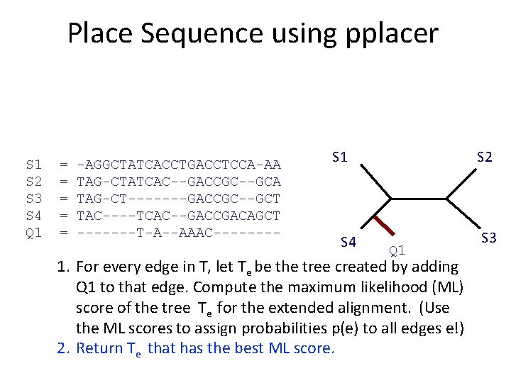
Place Sequence S 1 S 2 S 3 S 4 Q 1 = = = -AGGCTATCACCTGACCTCCA-AA TAG-CTATCAC--GACCGC--GCA TAG-CT-------GACCGC--GCT TAC----TCAC--GACCGACAGCT -------T-A--AAAC---- S 1 S 4 S 2 Q 1 S 3

Phylogenetic Placement

Marker-based Taxon Identification Fragmentary sequences from some gene ACCG CGAG CGG GGCT TAGA GGGGG TCGAG GGCG GGG • . ACCT Full-length sequences for same gene, and an alignment and a tree AGG. . . GCAT TAGC. . . CCA TAGA. . . CTT AGC. . . ACA ACT. . TAGA. . A

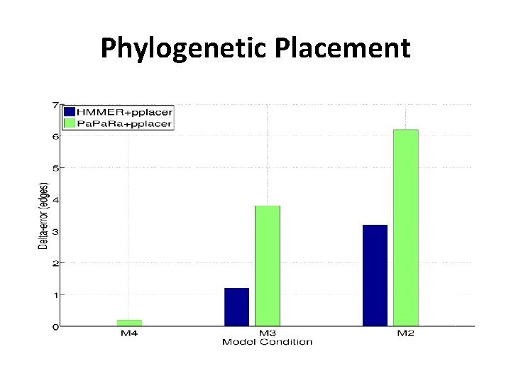
Phylogenetic Placement in 2011 • Align each query sequence to backbone alignment – HMMER (Finn et al. , NAR 2011) – Pa. Ra (Berger and Stamatakis, Bioinformatics 2011) • Place each query sequence into backbone tree – pplacer (Matsen et al. , BMC Bioinformatics, 2011) – EPA (Berger and Stamatakis, Systematic Biology 2011) Note: pplacer and EPA solve same problem (maximum likelihood placement under standard sequence evolution models)

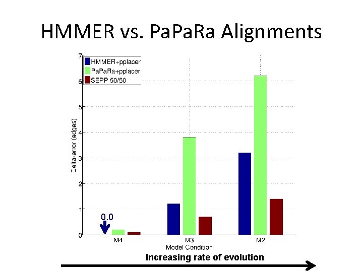
HMMER vs. Pa. Ra Alignments 0. 0 Increasing rate of evolution

What is HMMER+pplacer? • HMMER (Finn et al. , NAR 2011) (specifically, HMMAlign) is used to add the read s into the backbone alignment, thus producing an “extended alignment”. HMMAlign is based on profile Hidden Markov Models (profile HMMs). • pplacer (Matsen et al. BMC Bioinformatics 2010) is used to add read s into the best location in the tree T. pplacer is based on phylogenetic sequence evolution models (e. g. , GTR), and uses maximum likelihood.

A general topology for a profile HMM • • • D: deletion state I: insertion state M: match state (correspond to sites in the alignment) • Insertion and Match states emit letters (nucleotides, amino acids, other) from a distribution Edges have transition probabilities • • • From DOI: 10. 1109/ICPR. 2004. 1334187 A path through the profile HMM (with random selection of letters from D and I states) generates a sequence Given a sequence, you can find the maximum likelihood path through the model in polynomial time (dynamic programming)

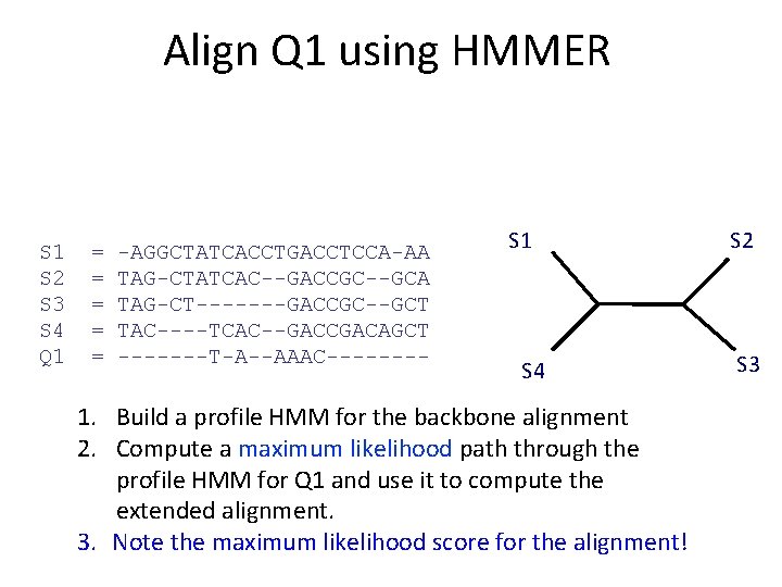
Profile Hidden Markov Models Profile HMMs are probabilistic generative models to represent multiple sequence alignments. HMMER software suite can • • • Build a profile HMM given a multiple sequence alignment A Use the profile HMM to add a sequence s into A, and return the “probability” that the HMM generated s (the “score”) Select between different profile HMMs based on score

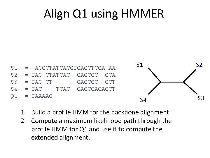
Input S 1 S 2 S 3 S 4 Q 1 = = = -AGGCTATCACCTGACCTCCA-AA TAG-CTATCAC--GACCGC--GCA TAG-CT-------GACCGC--GCT TAC----TCAC--GACCGACAGCT TAAAAC S 1 S 4 1. Build a profile HMM for the backbone alignment 2. Compute a maximum likelihood path through the profile HMM for Q 1 and use it to compute the extended alignment. S 2 S 3

Align Q 1 using HMMER S 1 S 2 S 3 S 4 Q 1 = = = -AGGCTATCACCTGACCTCCA-AA TAG-CTATCAC--GACCGC--GCA TAG-CT-------GACCGC--GCT TAC----TCAC--GACCGACAGCT TAAAAC S 1 S 4 1. Build a profile HMM for the backbone alignment 2. Compute a maximum likelihood path through the profile HMM for Q 1 and use it to compute the extended alignment. S 2 S 3

Align Q 1 using HMMER S 1 S 2 S 3 S 4 Q 1 = = = -AGGCTATCACCTGACCTCCA-AA TAG-CTATCAC--GACCGC--GCA TAG-CT-------GACCGC--GCT TAC----TCAC--GACCGACAGCT -------T-A--AAAC---- S 1 S 4 1. Build a profile HMM for the backbone alignment 2. Compute a maximum likelihood path through the profile HMM for Q 1 and use it to compute the extended alignment. 3. Note the maximum likelihood score for the alignment! S 2 S 3

Align Q 1 using HMMER S 1 S 2 S 3 S 4 Q 1 = = = -AGGCTATCACCTGACCTCCA-AA TAG-CTATCAC--GACCGC--GCA TAG-CT-------GACCGC--GCT TAC----TCAC--GACCGACAGCT -------T-A--AAAC---- S 1 S 4 1. Build a profile HMM for the backbone alignment 2. Compute a maximum likelihood path through the profile HMM for Q 1 and use it to compute the extended alignment. 3. Note the maximum likelihood score for the alignment! S 2 S 3

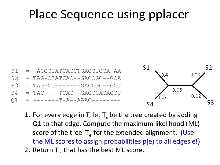
What is pplacer? • pplacer: software developed by Erick Matsen and colleagues. See http: //matsen. fhcrc. org/pplacer/ • Input: read s, alignment A (on S and s), tree on S • Output: – “Best” location to add s in T (under maximum likelihood). – For every edge e in T, the value p(e) for the probability for s being placed on e (these probabilities add up to 1)

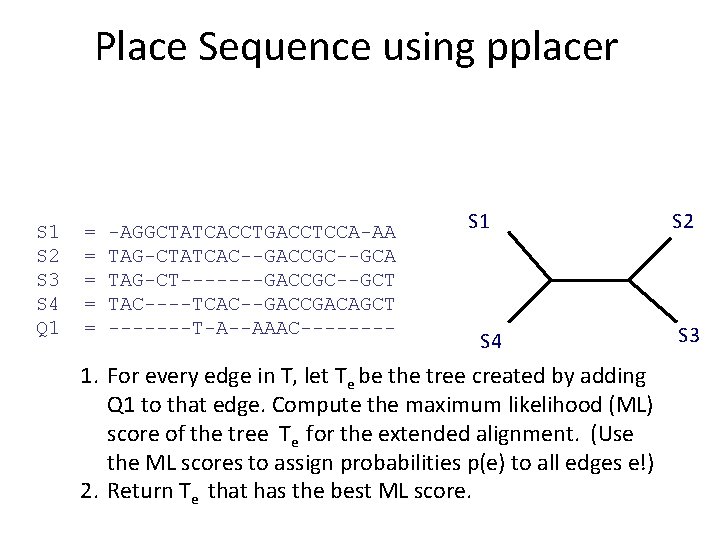
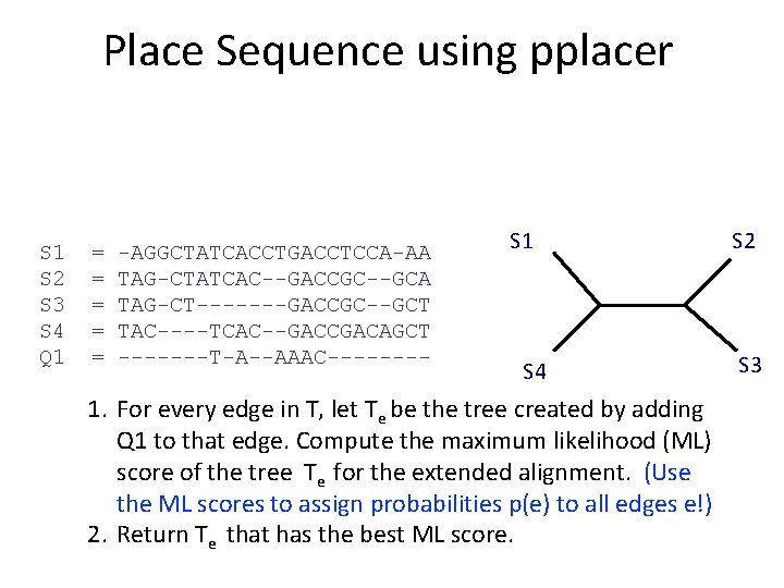
Place Sequence using pplacer S 1 S 2 S 3 S 4 Q 1 = = = -AGGCTATCACCTGACCTCCA-AA TAG-CTATCAC--GACCGC--GCA TAG-CT-------GACCGC--GCT TAC----TCAC--GACCGACAGCT -------T-A--AAAC---- S 1 S 4 1. For every edge in T, let Te be the tree created by adding Q 1 to that edge. Compute the maximum likelihood (ML) score of the tree Te for the extended alignment. (Use the ML scores to assign probabilities p(e) to all edges e!) 2. Return Te that has the best ML score. S 2 S 3

Place Sequence using pplacer S 1 S 2 S 3 S 4 Q 1 = = = -AGGCTATCACCTGACCTCCA-AA TAG-CTATCAC--GACCGC--GCA TAG-CT-------GACCGC--GCT TAC----TCAC--GACCGACAGCT -------T-A--AAAC---- S 1 S 4 1. For every edge in T, let Te be the tree created by adding Q 1 to that edge. Compute the maximum likelihood (ML) score of the tree Te for the extended alignment. (Use the ML scores to assign probabilities p(e) to all edges e!) 2. Return Te that has the best ML score. S 2 S 3

Place Sequence using pplacer S 1 S 2 S 3 S 4 Q 1 = = = -AGGCTATCACCTGACCTCCA-AA TAG-CTATCAC--GACCGC--GCA TAG-CT-------GACCGC--GCT TAC----TCAC--GACCGACAGCT -------T-A--AAAC---- S 1 0. 03 0. 4 0. 05 S 4 0. 5 0. 02 1. For every edge in T, let Te be the tree created by adding Q 1 to that edge. Compute the maximum likelihood (ML) score of the tree Te for the extended alignment. (Use the ML scores to assign probabilities p(e) to all edges e!) 2. Return Te that has the best ML score. S 2 S 3

Place Sequence using pplacer S 1 S 2 S 3 S 4 Q 1 = = = -AGGCTATCACCTGACCTCCA-AA TAG-CTATCAC--GACCGC--GCA TAG-CT-------GACCGC--GCT TAC----TCAC--GACCGACAGCT -------T-A--AAAC---- S 1 0. 03 0. 4 0. 05 S 4 0. 5 0. 02 1. For every edge in T, let Te be the tree created by adding Q 1 to that edge. Compute the maximum likelihood (ML) score of the tree Te for the extended alignment. (Use the ML scores to assign probabilities p(e) to all edges e!) 2. Return Te that has the best ML score. S 2 S 3

Place Sequence using pplacer S 1 S 2 S 3 S 4 Q 1 = = = -AGGCTATCACCTGACCTCCA-AA TAG-CTATCAC--GACCGC--GCA TAG-CT-------GACCGC--GCT TAC----TCAC--GACCGACAGCT -------T-A--AAAC---- S 1 0. 03 0. 4 0. 05 S 4 0. 5 0. 02 1. For every edge in T, let Te be the tree created by adding Q 1 to that edge. Compute the maximum likelihood (ML) score of the tree Te for the extended alignment. (Use the ML scores to assign probabilities p(e) to all edges e!) 2. Return Te that has the best ML score. S 2 S 3

Place Sequence using pplacer S 1 S 2 S 3 S 4 Q 1 = = = -AGGCTATCACCTGACCTCCA-AA TAG-CTATCAC--GACCGC--GCA TAG-CT-------GACCGC--GCT TAC----TCAC--GACCGACAGCT -------T-A--AAAC---- S 1 S 4 S 2 Q 1 1. For every edge in T, let Te be the tree created by adding Q 1 to that edge. Compute the maximum likelihood (ML) score of the tree Te for the extended alignment. (Use the ML scores to assign probabilities p(e) to all edges e!) 2. Return Te that has the best ML score. S 3

HMMER vs. Pa. Ra Alignments 0. 0 Increasing rate of evolution

SEPP vs. HMMER, Pa. Ra alignments 0. 0 Increasing rate of evolution

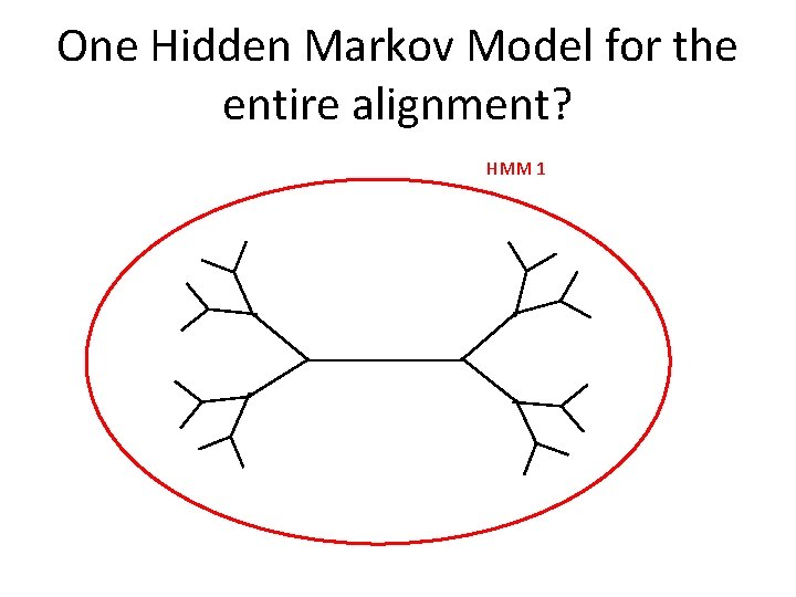
One Hidden Markov Model for the entire alignment? HMM 1

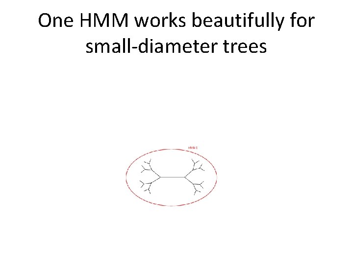
One HMM works beautifully for small-diameter trees

One HMM works poorly for large-diameter trees

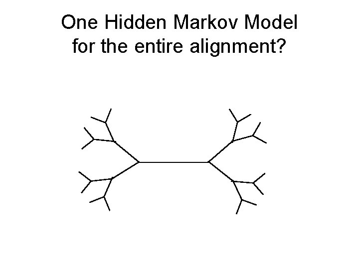
One Hidden Markov Model for the entire alignment?

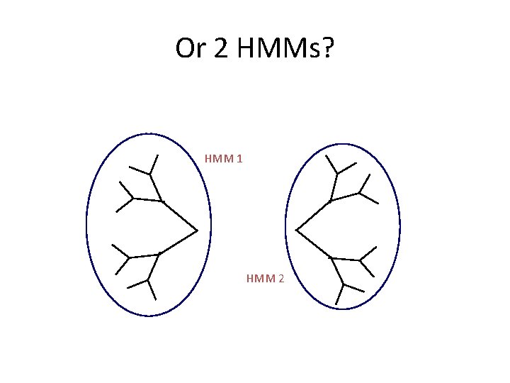
Or 2 HMMs? HMM 1 HMM 2

Or 4 HMMs? HMM 1 HMM 3 HMM 2 HMM 4

SEPP Ensemble of HMMs (e. HMMs) • Construct an e. HMM, given an alignment A and tree T on A: – Divide the leaves of T into subsets (by deleting centroid edges) until every subset is small enough – Build a profile HMM on each subset using HMMER

SEPP Design To insert query sequence Q 1 into backbone tree T • • Represent the backbone MSA with an e. HMM, based on maximum alignment subset size Score Q 1 against every profile HMM in the collection The best scoring HMM is used to compute the extended alignment Use pplacer on the extended alignment to add Q 1 into tree T (restricted to subtree based on maximum placement subset size)

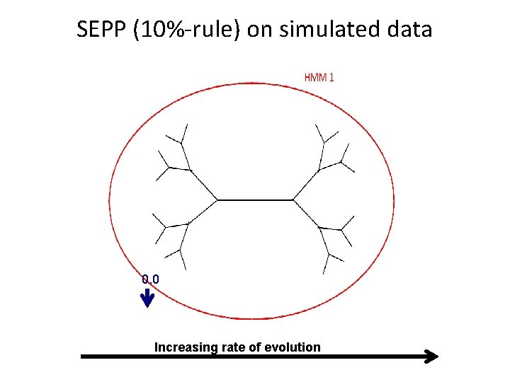
SEPP Parameter Exploration § § § Alignment subset size and placement subset size impact the accuracy: § Small alignment subset sizes best § Large placement subset size best But running time and memory problems… Compromise 10% rule (both subset sizes 10% of backbone) had best overall performance

SEPP (10%-rule) on simulated data 0. 0 Increasing rate of evolution

The Tutorial (by Mike Nute) • PASTA for large-scale MSA and tree estimation • SEPP for taxon ID – Will show you how to run SEPP – Will show you how to use branch lengths in SEPP’s placement of reads to get interesting insights • TIPP for taxon ID and abundance profiling

TIPP https: //github. com/smirarab/sepp TIPP (Bioinformatics 2014) performs marker gene-based: • taxonomic identification (what is this read? ) and • metagenomic abundance profiling (at some taxonomic level) TIPP uses • PASTA (J. Comp. Biol. 2015) to compute large-scale multiple sequence alignments (one for each marker gene) and • SEPP (Pacific Symposium on Biocomputing 2012) to add short reads into refined taxonomies (one for each marker gene)

High indel datasets containing known genomes Note: NBC, Meta. Phl. An, and Meta. Phyler cannot classify any sequences from at least one of the high indel long sequence datasets, and m. OTU terminates with an error message on all the high indel datasets.

“Novel” genome datasets Note: m. OTU terminates with an error message on the long fragment datasets and high indel datasets.

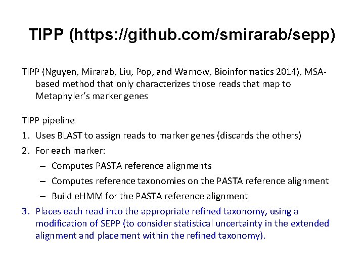
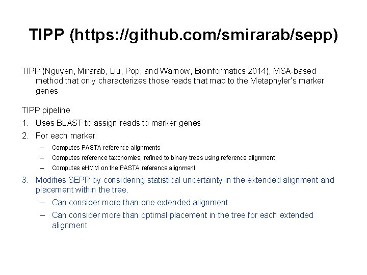
TIPP (https: //github. com/smirarab/sepp) TIPP (Nguyen, Mirarab, Liu, Pop, and Warnow, Bioinformatics 2014), MSAbased method that only characterizes those reads that map to Metaphyler’s marker genes TIPP pipeline 1. Uses BLAST to assign reads to marker genes (discards the others) 2. For each marker: – Computes PASTA reference alignments – Computes reference taxonomies on the PASTA reference alignment – Build e. HMM for the PASTA reference alignment 3. Places each read into the appropriate refined taxonomy, using a modification of SEPP (to consider statistical uncertainty in the extended alignment and placement within the refined taxonomy). – Can consider more than one extended alignment – Can consider more than optimal placement in the tree for each extended

TIPP for Taxonomic ID – output file

54100 = NCBI taxon ID

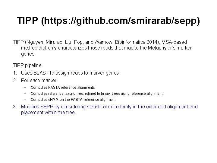
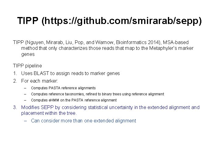
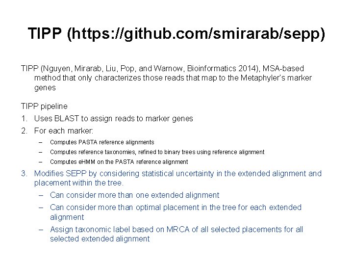
TIPP (https: //github. com/smirarab/sepp) TIPP (Nguyen, Mirarab, Liu, Pop, and Warnow, Bioinformatics 2014), MSA-based method that only characterizes those reads that map to the Metaphyler’s marker genes TIPP pipeline 1. Uses BLAST to assign reads to marker genes 2. For each marker: – Computes PASTA reference alignments – Computes reference taxonomies, refined to binary trees using reference alignment – Computes e. HMM on the PASTA reference alignment 3. Modifies SEPP by considering statistical uncertainty in the extended alignment and placement within the tree. – Can consider more than one extended alignment – Can consider more than optimal placement in the tree for each extended alignment – Assign taxonomic label based on MRCA of all selected placements for all selected extended alignment

TIPP (https: //github. com/smirarab/sepp) TIPP (Nguyen, Mirarab, Liu, Pop, and Warnow, Bioinformatics 2014), MSA-based method that only characterizes those reads that map to the Metaphyler’s marker genes TIPP pipeline 1. Uses BLAST to assign reads to marker genes 2. For each marker: – Computes PASTA reference alignments – Computes reference taxonomies, refined to binary trees using reference alignment – Computes e. HMM on the PASTA reference alignment 3. Modifies SEPP by considering statistical uncertainty in the extended alignment and placement within the tree. – Can consider more than one extended alignment – Can consider more than optimal placement in the tree for each extended alignment – Assign taxonomic label based on MRCA of all selected placements for all selected extended alignment

TIPP (https: //github. com/smirarab/sepp) TIPP (Nguyen, Mirarab, Liu, Pop, and Warnow, Bioinformatics 2014), MSA-based method that only characterizes those reads that map to the Metaphyler’s marker genes TIPP pipeline 1. Uses BLAST to assign reads to marker genes 2. For each marker: – Computes PASTA reference alignments – Computes reference taxonomies, refined to binary trees using reference alignment – Computes e. HMM on the PASTA reference alignment 3. Modifies SEPP by considering statistical uncertainty in the extended alignment and placement within the tree. – Can consider more than one extended alignment – Can consider more than optimal placement in the tree for each extended alignment – Assign taxonomic label based on MRCA of all selected placements for all selected extended alignment

TIPP (https: //github. com/smirarab/sepp) TIPP (Nguyen, Mirarab, Liu, Pop, and Warnow, Bioinformatics 2014), MSA-based method that only characterizes those reads that map to the Metaphyler’s marker genes TIPP pipeline 1. Uses BLAST to assign reads to marker genes 2. For each marker: – Computes PASTA reference alignments – Computes reference taxonomies, refined to binary trees using reference alignment – Computes e. HMM on the PASTA reference alignment 3. Modifies SEPP by considering statistical uncertainty in the extended alignment and placement within the tree. – Can consider more than one extended alignment – Can consider more than optimal placement in the tree for each extended alignment – Assign taxonomic label based on MRCA of all selected placements for all selected extended alignment

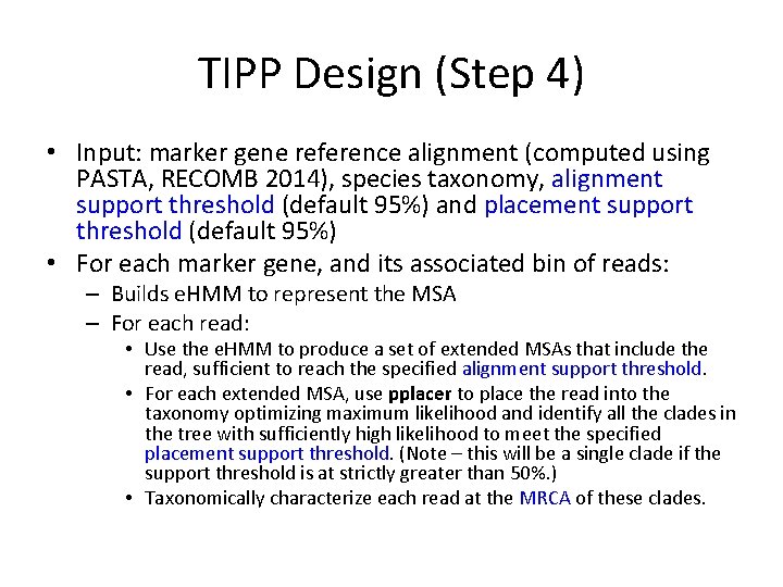
TIPP Design (Step 4) • Input: marker gene reference alignment (computed using PASTA, RECOMB 2014), species taxonomy, alignment support threshold (default 95%) and placement support threshold (default 95%) • For each marker gene, and its associated bin of reads: – Builds e. HMM to represent the MSA – For each read: • Use the e. HMM to produce a set of extended MSAs that include the read, sufficient to reach the specified alignment support threshold. • For each extended MSA, use pplacer to place the read into the taxonomy optimizing maximum likelihood and identify all the clades in the tree with sufficiently high likelihood to meet the specified placement support threshold. (Note – this will be a single clade if the support threshold is at strictly greater than 50%. ) • Taxonomically characterize each read at the MRCA of these clades.

TIPP Design (Step 4) • Input: marker gene reference alignment (computed using PASTA, RECOMB 2014), species taxonomy, alignment support threshold (default 95%) and placement support threshold (default 95%) • For each marker gene, and its associated bin of reads: – Builds e. HMM to represent the MSA – For each read: • Use the e. HMM to produce a set of extended MSAs that include the read, sufficient to reach the specified alignment support threshold. • For each extended MSA, use pplacer to place the read into the taxonomy optimizing maximum likelihood and identify all the clades in the tree with sufficiently high likelihood to meet the specified placement support threshold. (Note – this will be a single clade if the support threshold is at strictly greater than 50%. ) • Taxonomically characterize each read at the MRCA of these clades.

TIPP Design (Step 4) • Input: marker gene reference alignment (computed using PASTA, RECOMB 2014), species taxonomy, alignment support threshold (default 95%) and placement support threshold (default 95%) • For each marker gene, and its associated bin of reads: – Builds e. HMM to represent the MSA – For each read: • Use the e. HMM to produce a set of extended MSAs that include the read, sufficient to reach the specified alignment support threshold. • For each extended MSA, use pplacer to place the read into the taxonomy optimizing maximum likelihood and identify all the clades in the tree with sufficiently high likelihood to meet the specified placement support threshold. (Note – this will be a single clade if the support threshold is at strictly greater than 50%. ) • Taxonomically characterize each read at the MRCA of these clades.

TIPP Design (Step 4) • Input: marker gene reference alignment (computed using PASTA, RECOMB 2014), species taxonomy, alignment support threshold (default 95%) and placement support threshold (default 95%) • For each marker gene, and its associated bin of reads: – Builds e. HMM to represent the MSA – For each read: • Use the e. HMM to produce a set of extended MSAs that include the read, sufficient to reach the specified alignment support threshold. • For each extended MSA, use pplacer to place the read into the taxonomy optimizing maximum likelihood and identify all the clades in the tree with sufficiently high likelihood to meet the specified placement support threshold. (Note – this will be a single clade if the support threshold is at strictly greater than 50%. ) • Taxonomically characterize each read at the MRCA of these clades.

TIPP Design (Step 4) • Input: marker gene reference alignment (computed using PASTA, RECOMB 2014), species taxonomy, alignment support threshold (default 95%) and placement support threshold (default 95%) • For each marker gene, and its associated bin of reads: – Builds e. HMM to represent the MSA – For each read: • Use the e. HMM to produce a set of extended MSAs that include the read, sufficient to reach the specified alignment support threshold. • For each extended MSA, use pplacer to place the read into the taxonomy optimizing maximum likelihood and identify all the clades in the tree with sufficiently high likelihood to meet the specified placement support threshold. (Note – this will be a single clade if the support threshold is at strictly greater than 50%. ) • Taxonomically characterize each read at the MRCA of these clades.

TIPP Design (Step 4) • Input: marker gene reference alignment (computed using PASTA, RECOMB 2014), species taxonomy, alignment support threshold (default 95%) and placement support threshold (default 95%) • For each marker gene, and its associated bin of reads: – Builds e. HMM to represent the MSA – For each read: • Use the e. HMM to produce a set of extended MSAs that include the read, sufficient to reach the specified alignment support threshold. • For each extended MSA, use pplacer to place the read into the taxonomy optimizing maximum likelihood and identify all the clades in the tree with sufficiently high likelihood to meet the specified placement support threshold. (Note – this will be a single clade if the support threshold is at strictly greater than 50%. ) • Taxonomically characterize each read at the MRCA of these clades.

TIPP Design (Step 4) • Input: marker gene reference alignment (computed using PASTA, RECOMB 2014), species taxonomy, alignment support threshold (default 95%) and placement support threshold (default 95%) • For each marker gene, and its associated bin of reads: – Builds e. HMM to represent the MSA – For each read: • Use the e. HMM to produce a set of extended MSAs that include the read, sufficient to reach the specified alignment support threshold. • For each extended MSA, use pplacer to place the read into the taxonomy optimizing maximum likelihood and identify all the clades in the tree with sufficiently high likelihood to meet the specified placement support threshold. (Note – this will be a single clade if the support threshold is at strictly greater than 50%. ) • Taxonomically characterize each read at the MRCA of these clades.

The Tutorial (by Mike Nute) • PASTA for large-scale MSA and tree estimation • SEPP for taxon ID – Will show you how to run SEPP – Will show you how to use branch lengths in SEPP’s placement of reads to get interesting insights • TIPP for taxon ID and abundance profiling

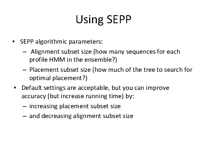
Using SEPP • SEPP algorithmic parameters: – Alignment subset size (how many sequences for each profile HMM in the ensemble? ) – Placement subset size (how much of the tree to search for optimal placement? ) • Default settings are acceptable, but you can improve accuracy (but increase running time) by: – increasing placement subset size – and decreasing alignment subset size

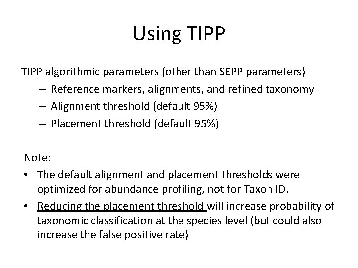
Using TIPP algorithmic parameters (other than SEPP parameters) – Reference markers, alignments, and refined taxonomy – Alignment threshold (default 95%) – Placement threshold (default 95%) Note: • The default alignment and placement thresholds were optimized for abundance profiling, not for Taxon ID. • Reducing the placement threshold will increase probability of taxonomic classification at the species level (but could also increase the false positive rate)

Using PASTA • Main algorithmic parameters in PASTA: – Decomposition edge – Alignment subset size – Subset aligner – Alignment merger – Tree estimator and ML model – Number of iterations • Note: type of data (AA or nucleotide) affects subset alignment method (e. g. , Muscle is particularly bad choice for AA but not too bad for DNA, MAFFT L-INS-i among best for both) • Ask Mike about using BAli-Phy (Bayesian alignment estimation method) within PASTA

TIPP is under development! • We are modifying TIPP’s design to improve taxonomic identification and abundance profiling on shotgun sequencing data • Stay tuned! Developers: Erin Molloy, Mike Nute, Nidhi Shah, Mihai Pop, and Tandy Warnow

Profile HMMs vs. e. HMMs An e. HMM is better able to: • detect homology between full length sequences and fragmentary sequences • add fragmentary sequences into an existing alignment especially when there are many indels and/or substitutions (e. g. , in the twilight zone)

Our Publications using e. HMMs • S. Mirarab, N. Nguyen, and T. Warnow. "SEPP: SATé-Enabled Phylogenetic Placement. " Proceedings of the 2012 Pacific Symposium on Biocomputing (PSB 2012) 17: 247 -258. • N. Nguyen, S. Mirarab, B. Liu, M. Pop, and T. Warnow "TIPP: Taxonomic Identification and Phylogenetic Profiling. " Bioinformatics (2014) 30(24): 35483555. • N. Nguyen, S. Mirarab, K. Kumar, and T. Warnow, "Ultra-large alignments using phylogeny aware profiles". Proceedings RECOMB 2015 and Genome Biology (2015) 16: 124 • N. Nguyen, M. Nute, S. Mirarab, and T. Warnow, HIPPI: Highly accurate protein family classification with ensembles of HMMs. BMC Genomics (2016): 17 (Suppl 10): 765 All codes are available in open source form at https: //github. com/smirarab/sepp

Acknowledgments Ph. D students: Nam Nguyen (now postdoc at UCSD), Siavash Mirarab (now faculty at UCSD), Bo Liu (now at Square), Erin Molloy, Nidhi Shah (Maryland), and Mike Nute Mihai Pop, University of Maryland NSF grants to TW: DBI: 1062335, DEB 0733029, III: AF: 1513629 NIH grant to MP: R 01 -A 1 -100947 Also: Guggenheim Foundation Fellowship (to TW), Microsoft Research New England (to TW), David Bruton Jr. Centennial Professorship (to TW), Grainger Foundation (to TW), HHMI Predoctoral Fellowship (to SM) TACC, UTCS, and UIUC computational resources