2 4 Exact Equations 2 4 1 first

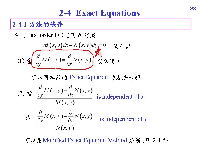
2 -4 Exact Equations 2 -4 -1 方法的條件 任何 first order DE 皆可改寫成 的型態 (1) 當 成立時， 可以用本節的 Exact Equation 的方法來解 (2) 當 或 is independent of x is independent of y 可以用Modified Exact Equation Method 來解 (見 2 -4 -5) 98

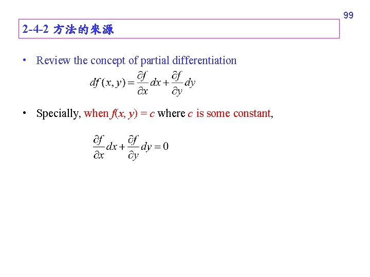
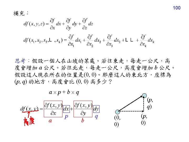
99 2 -4 -2 方法的來源 • Review the concept of partial differentiation • Specially, when f(x, y) = c where c is some constant,

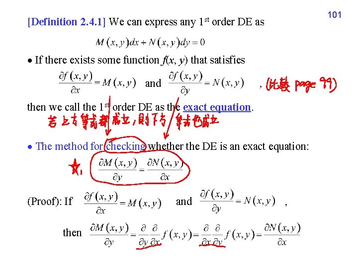
[Definition 2. 4. 1] We can express any 1 st order DE as If there exists some function f(x, y) that satisfies and , then we call the 1 st order DE as the exact equation. The method for checking whether the DE is an exact equation: (Proof): If and , then 101

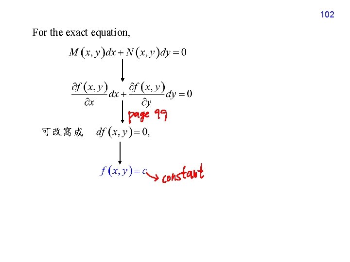
102 For the exact equation, 可改寫成

103 2 -4 -3 解法 The method for solving the exact equation (A): (1) g(y) is a constant for x (3) (2) (3) 代入 (2) (4) further computation Solution

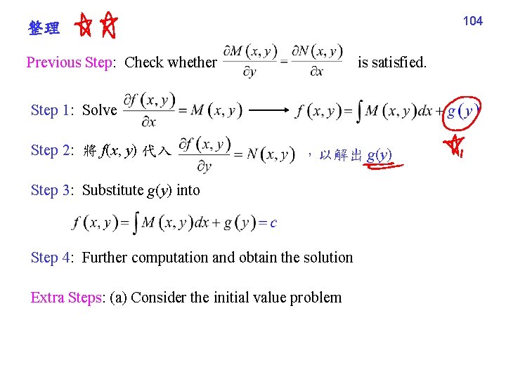
104 整理 Previous Step: Check whether is satisfied. Step 1: Solve Step 2: 將 f(x, y) 代入 ，以解出 g(y) Step 3: Substitute g(y) into Step 4: Further computation and obtain the solution Extra Steps: (a) Consider the initial value problem

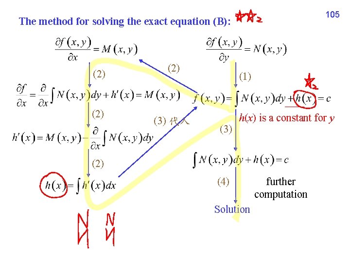
105 The method for solving the exact equation (B): (2) (2) (3) 代入 (1) (3) h(x) is a constant for y (2) (4) Solution further computation

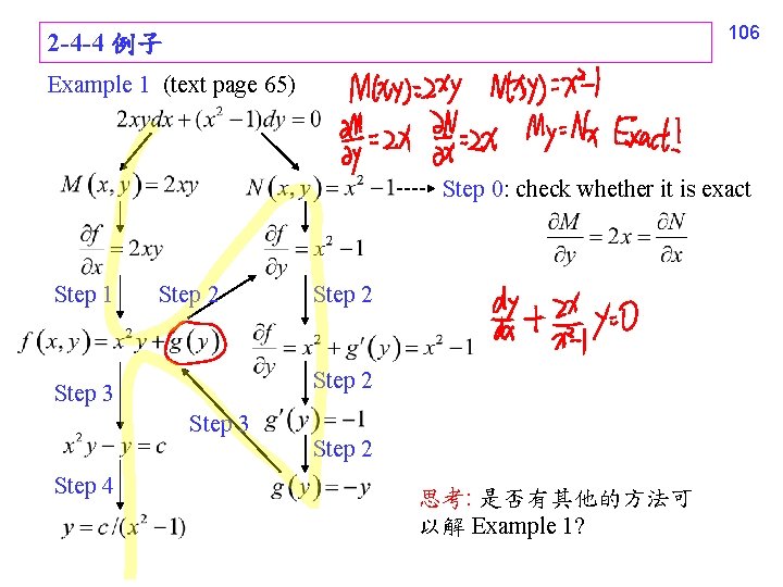
106 2 -4 -4 例子 Example 1 (text page 65) Step 0: check whether it is exact Step 1 Step 2 Step 3 Step 4 Step 2 思考: 是否有其他的方法可 以解 Example 1?

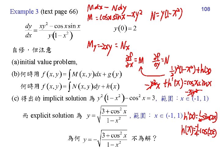
108 Example 3 (text page 66) 自修，但注意 (a) initial value problem, (b) 何時用 (c) 得出的 implicit solution 為 而 explicit solution 為 , 範圍：x (-1, 1) , 範圍： x (-1, 1) 為何 不為解？

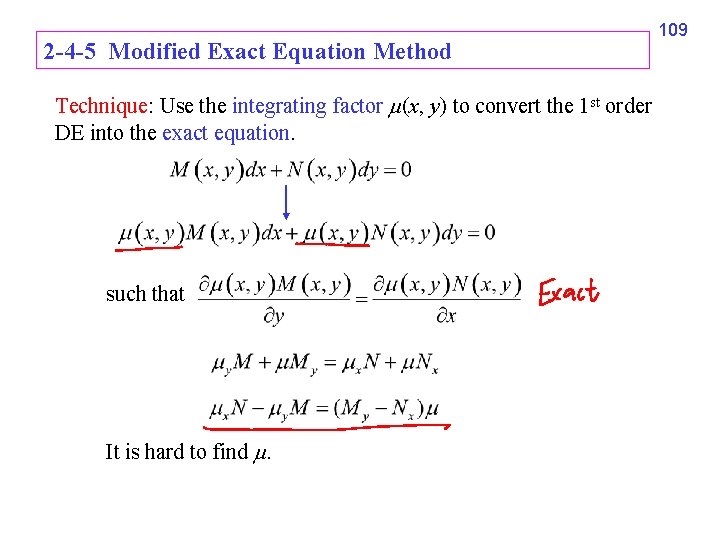
2 -4 -5 Modified Exact Equation Method Technique: Use the integrating factor (x, y) to convert the 1 st order DE into the exact equation. such that It is hard to find . 109

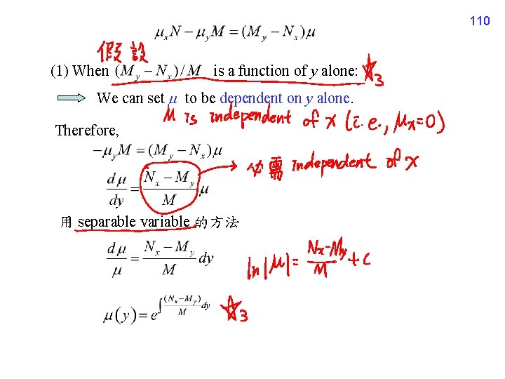
110 (1) When is a function of y alone: We can set to be dependent on y alone. Therefore, 用 separable variable 的方法

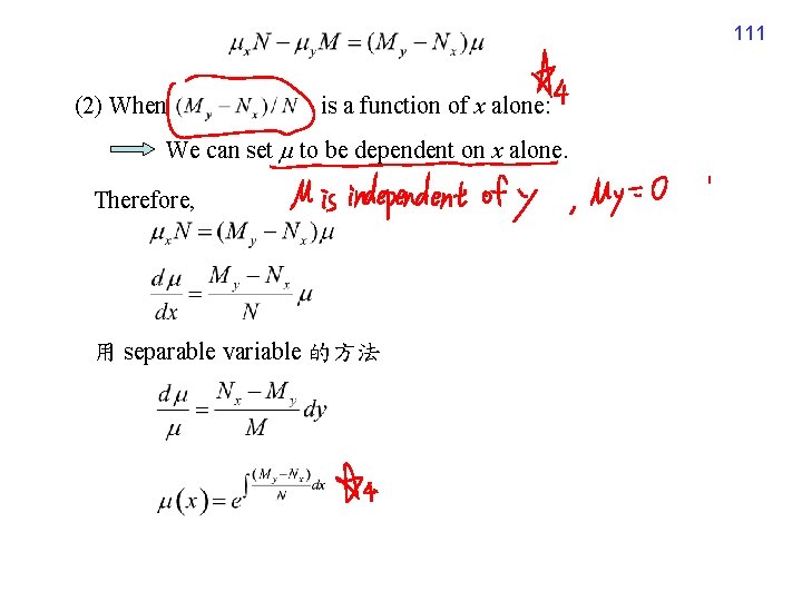
111 (2) When is a function of x alone: We can set to be dependent on x alone. Therefore, 用 separable variable 的方法

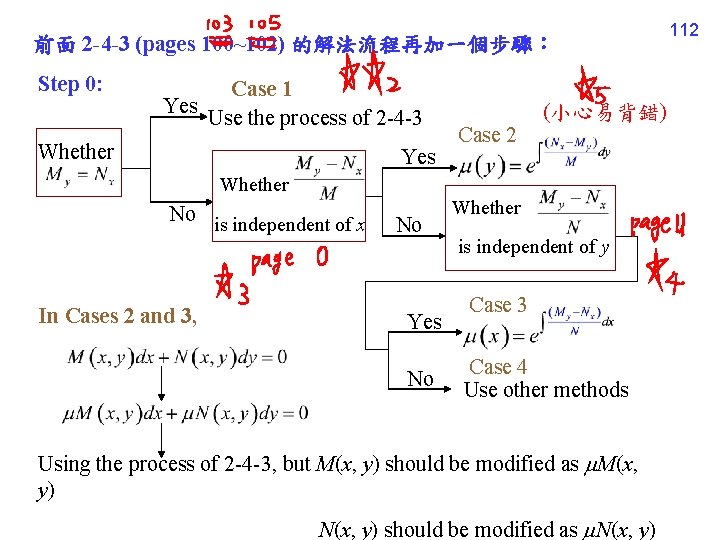
前面 2 -4 -3 (pages 100~102) 的解法流程再加一個步驟： Step 0: Case 1 Yes Use the process of 2 -4 -3 Whether Yes Case 2 (小心易背錯) Whether No is independent of x In Cases 2 and 3, No Yes No Whether is independent of y Case 3 Case 4 Use other methods Using the process of 2 -4 -3, but M(x, y) should be modified as M(x, y) N(x, y) should be modified as N(x, y) 112

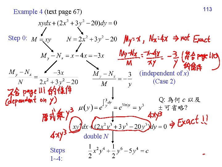
113 Example 4 (text page 67) Step 0: (independent of x) (Case 2) Q: 為何 c 以及 可省略? double N Steps 1~4:

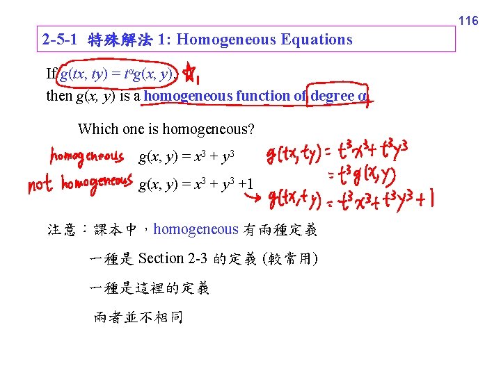
116 2 -5 -1 特殊解法 1: Homogeneous Equations If g(tx, ty) = tαg(x, y), then g(x, y) is a homogeneous function of degree α. Which one is homogeneous? g(x, y) = x 3 + y 3 +1 注意：課本中，homogeneous 有兩種定義 一種是 Section 2 -3 的定義 (較常用) 一種是這裡的定義 兩者並不相同

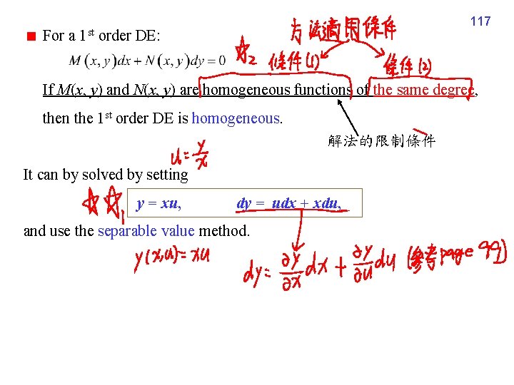
117 For a 1 st order DE: If M(x, y) and N(x, y) are homogeneous functions of the same degree, then the 1 st order DE is homogeneous. 解法的限制條件 It can by solved by setting y = xu, dy = udx + xdu, and use the separable value method.

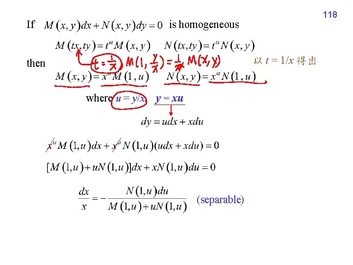
118 If is homogeneous 以 t = 1/x 得出 then where u = y/x, y = xu (separable)

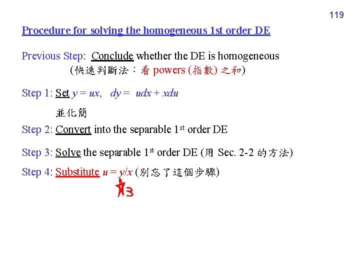
119 Procedure for solving the homogeneous 1 st order DE Previous Step: Conclude whether the DE is homogeneous (快速判斷法：看 powers (指數) 之和) Step 1: Set y = ux, dy = udx + xdu 並化簡 Step 2: Convert into the separable 1 st order DE Step 3: Solve the separable 1 st order DE (用 Sec. 2 -2 的方法) Step 4: Substitute u = y/x (別忘了這個步驟)

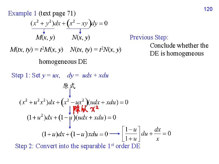
120 Example 1 (text page 71) M(x, y) N(x, y) M(tx, ty) = t 2 M(x, y) N(tx, ty) = t 2 N(x, y) Previous Step: Conclude whether the DE is homogeneous DE Step 1: Set y = ux, dy = udx + xdu 原式 Step 2: Convert into the separable 1 st order DE

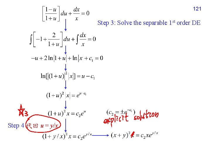
121 Step 3: Solve the separable 1 st order DE Step 4 代回 u = y/x

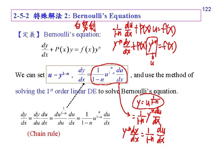
2 -5 -2 特殊解法 2: Bernoulli’s Equations 【定義】 Bernoulli’s equation: We can set u = y 1–n , , and use the method of solving the 1 st order linear DE to solve Bernoulli’s equation. (Chain rule) 122

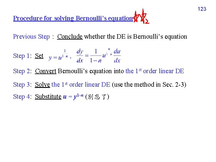
123 Procedure for solving Bernoulli’s equation Previous Step : Conclude whether the DE is Bernoulli’s equation Step 1: Set , Step 2: Convert Bernoulli’s equation into the 1 st order linear DE Step 3: Solve the 1 st order linear DE (use the method in Sec. 2 -3) Step 4: Substitute u = y 1–n (別忘了)

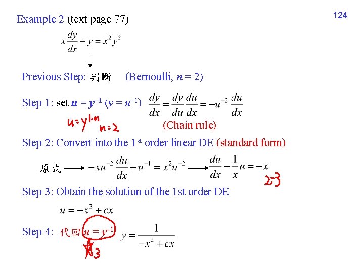
124 Example 2 (text page 77) Previous Step: 判斷 (Bernoulli, n = 2) Step 1: set u = y– 1 (y = u– 1) (Chain rule) Step 2: Convert into the 1 st order linear DE (standard form) 原式 Step 3: Obtain the solution of the 1 st order DE Step 4: 代回 u = y– 1

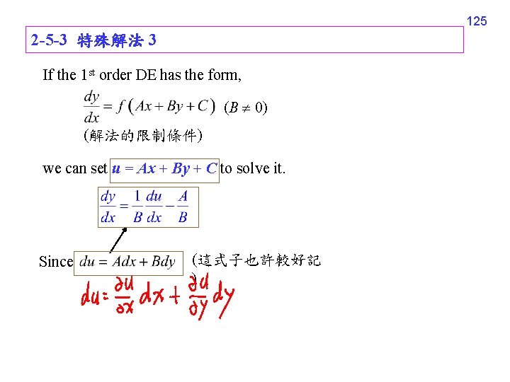
125 2 -5 -3 特殊解法 3 If the 1 st order DE has the form, (B 0) (解法的限制條件) we can set u = Ax + By + C to solve it. Since (這式子也許較好記 )

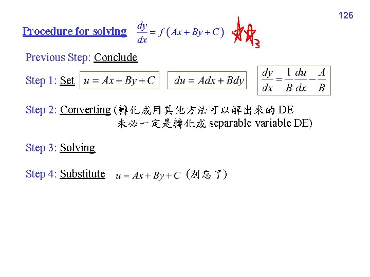
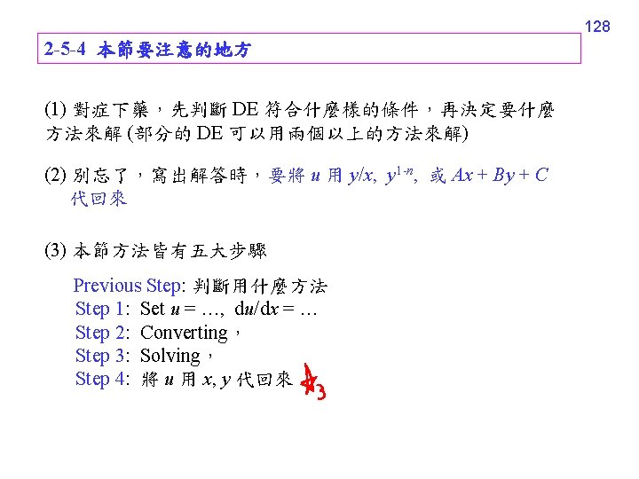
126 Procedure for solving Previous Step: Conclude Step 1: Set Step 2: Converting (轉化成用其他方法可以解出來的 DE 未必一定是轉化成 separable variable DE) Step 3: Solving Step 4: Substitute (別忘了)

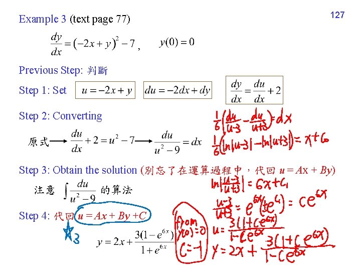
Example 3 (text page 77) 127 , Previous Step: 判斷 Step 1: Set Step 2: Converting 原式 Step 3: Obtain the solution (別忘了在運算過程中，代回 u = Ax + By) 注意 的算法 Step 4: 代回 u = Ax + By +C

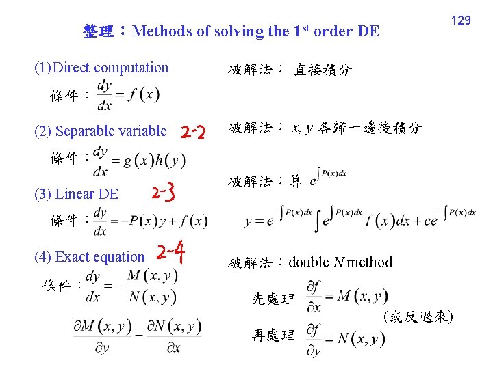
整理：Methods of solving the (1) Direct computation 1 st 129 order DE 破解法： 直接積分 條件： (2) Separable variable 破解法： x, y 各歸一邊後積分 條件： (3) Linear DE 條件： (4) Exact equation 條件： 破解法：算 破解法：double N method 先處理 (或反過來) 再處理

(4 -1) Exact equation 變型 130 破解法： 條件： is exact independent of x (4 -2) Exact equation 變型 破解法： 條件： is exact independent of y (5) Homogeneous equation 破解法：u = y/x, (y = xu) 條件： 再用 separable variable method

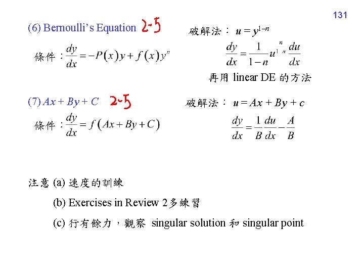
131 (6) Bernoulli’s Equation 破解法： u = y 1–n 條件： 再用 linear DE 的方法 (7) Ax + By + C 破解法： u = Ax + By + c 條件： 注意 (a) 速度的訓練 (b) Exercises in Review 2多練習 (c) 行有餘力，觀察 singular solution 和 singular point

132 練習 Sec. 2 -4: 3, 17, 25, 29, 32, 35, 38 Sec. 2 -5: 3, 5, 14, 17, 20, 22, 24, 25, 29 Chap. 2 Review: 2, 5 , 8, 9, 10, 11, 14, 15, 16, 19

133 Chapter 4 Higher Order Differential Equations Highest differentiation: , n > 1 Most of the methods in Chapter 4 are applied for the linear DE.

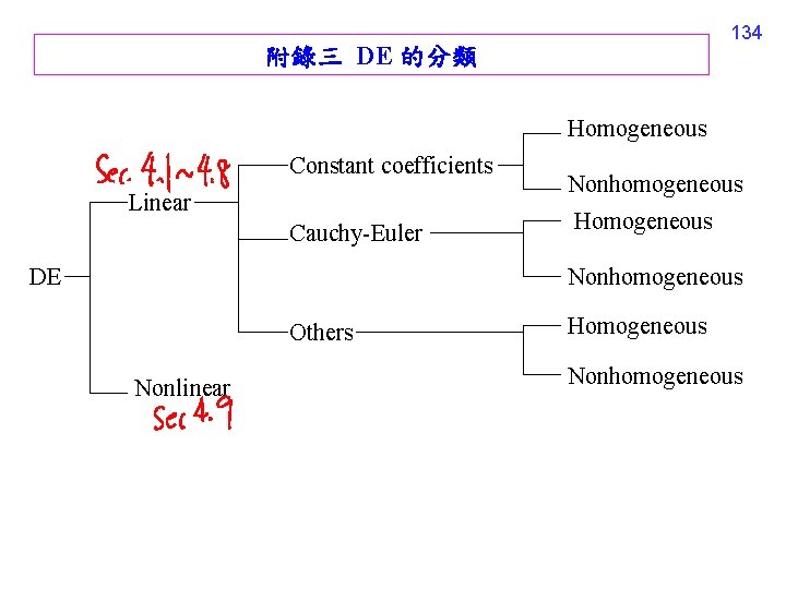
134 附錄三 DE 的分類 Homogeneous Constant coefficients Linear Cauchy-Euler DE Nonhomogeneous Homogeneous Nonhomogeneous Others Nonlinear Homogeneous Nonhomogeneous

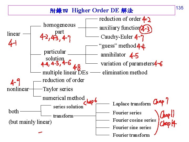
附錄四 Higher Order DE 解法 linear homogeneous particular solution multiple linear DEs reduction of order nonlinear reduction of order auxiliary function Cauchy-Euler “guess” method annihilator variation of parameters elimination method Taylor series numerical method both (but mainly linear) series solution transform Laplace transform Fourier series Fourier cosine series Fourier transform 135

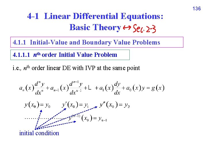
4 -1 Linear Differential Equations: Basic Theory 4. 1. 1 Initial-Value and Boundary Value Problems 4. 1. 1. 1 nth order Initial Value Problem i. e. , nth order linear DE with IVP at the same point ………………. . initial condition 136

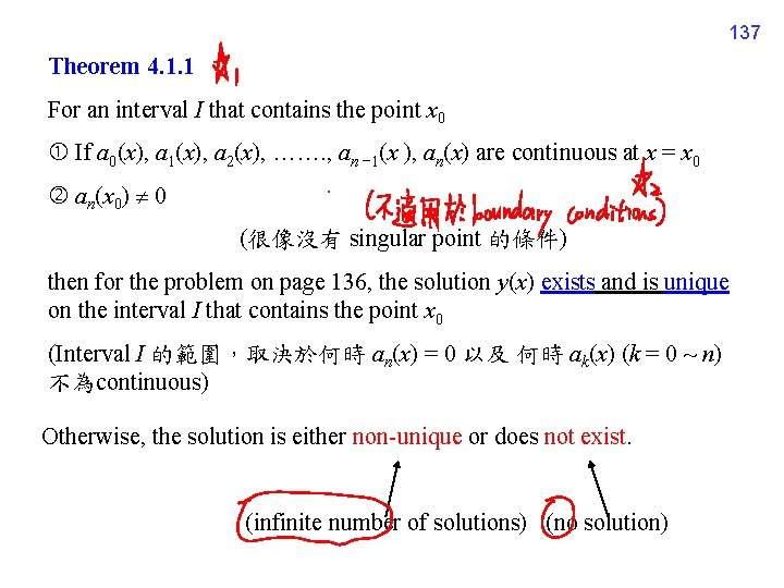
137 Theorem 4. 1. 1 For an interval I that contains the point x 0 If a 0(x), a 1(x), a 2(x), ……. , an − 1(x ), an(x) are continuous at x = x 0 an(x 0) 0 (很像沒有 singular point 的條件) then for the problem on page 136, the solution y(x) exists and is unique on the interval I that contains the point x 0 (Interval I 的範圍，取決於何時 an(x) = 0 以及 何時 ak(x) (k = 0 ~ n) 不為continuous) Otherwise, the solution is either non-unique or does not exist. (infinite number of solutions) (no solution)

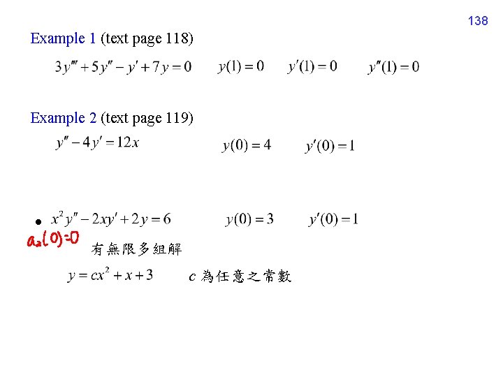
138 Example 1 (text page 118) Example 2 (text page 119) 有無限多組解 c 為任意之常數

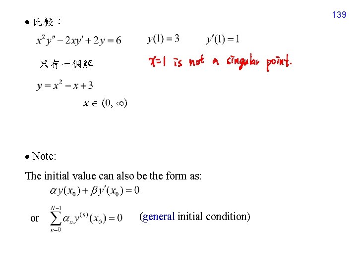
139 比較： 只有一個解 x (0, ) Note: The initial value can also be the form as: (general initial condition) or

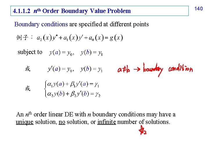
4. 1. 1. 2 nth Order Boundary Value Problem Boundary conditions are specified at different points 例子： subject to 或 或 An nth order linear DE with n boundary conditions may have a unique solution, no solution, or infinite number of solutions. 140

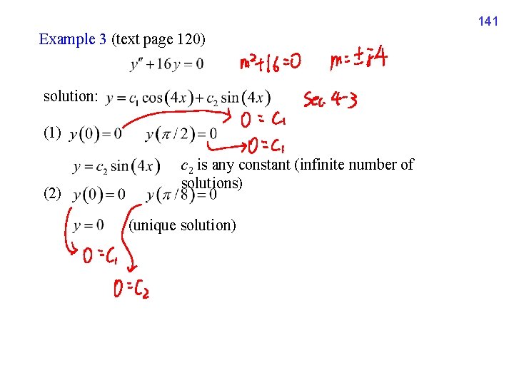
141 Example 3 (text page 120) solution: (1) (2) c 2 is any constant (infinite number of solutions) (unique solution)

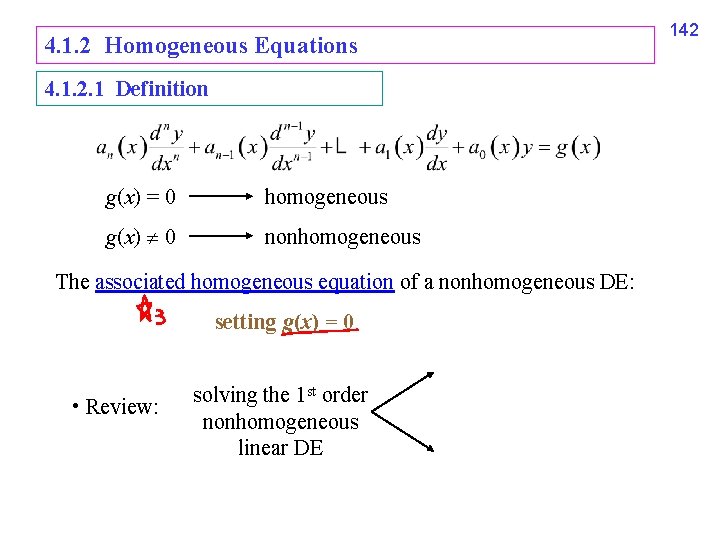
4. 1. 2 Homogeneous Equations 4. 1. 2. 1 Definition g(x) = 0 homogeneous g(x) 0 nonhomogeneous The associated homogeneous equation of a nonhomogeneous DE: setting g(x) = 0 • Review: solving the 1 st order nonhomogeneous linear DE 142

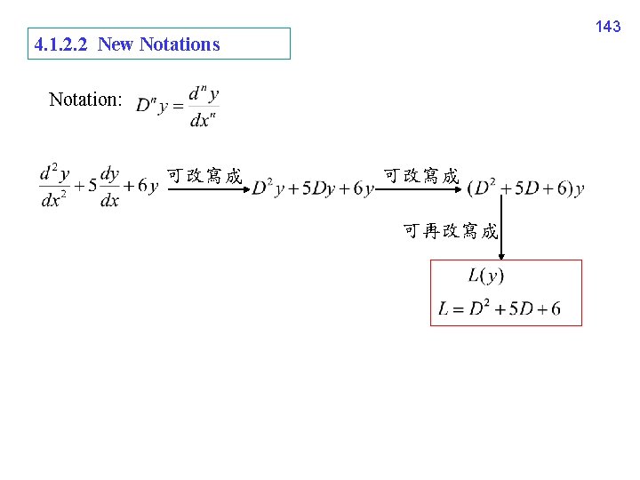
143 4. 1. 2. 2 New Notations Notation: 可改寫成 可再改寫成

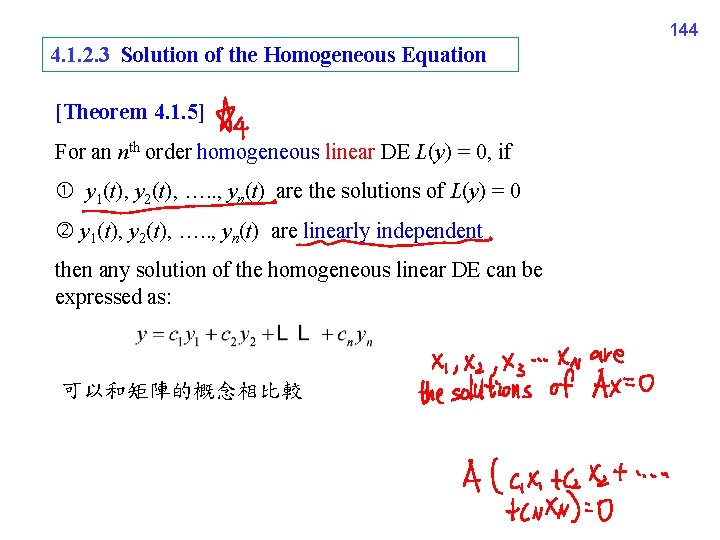
144 4. 1. 2. 3 Solution of the Homogeneous Equation [Theorem 4. 1. 5] For an nth order homogeneous linear DE L(y) = 0, if y 1(t), y 2(t), …. . , yn(t) are the solutions of L(y) = 0 y 1(t), y 2(t), …. . , yn(t) are linearly independent then any solution of the homogeneous linear DE can be expressed as: 可以和矩陣的概念相比較

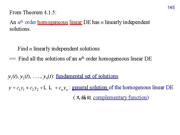
145 From Theorem 4. 1. 5: An nth order homogeneous linear DE has n linearly independent solutions. Find n linearly independent solutions == Find all the solutions of an nth order homogeneous linear DE y 1(t), y 2(t), …. . , yn(t): fundamental set of solutions : general solution of the homogenous linear DE (又稱做 complementary function)

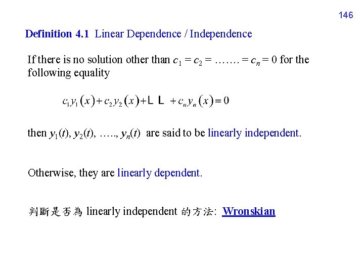
146 Definition 4. 1 Linear Dependence / Independence If there is no solution other than c 1 = c 2 = ……. = cn = 0 for the following equality then y 1(t), y 2(t), …. . , yn(t) are said to be linearly independent. Otherwise, they are linearly dependent. 判斷是否為 linearly independent 的方法: Wronskian

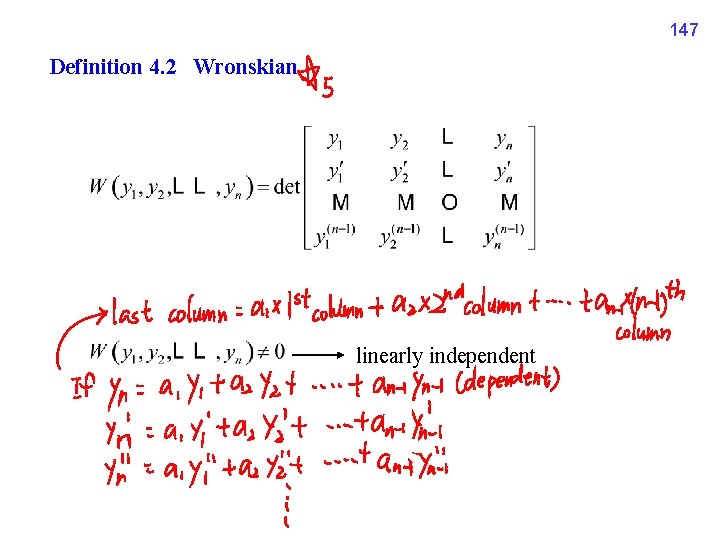
147 Definition 4. 2 Wronskian linearly independent

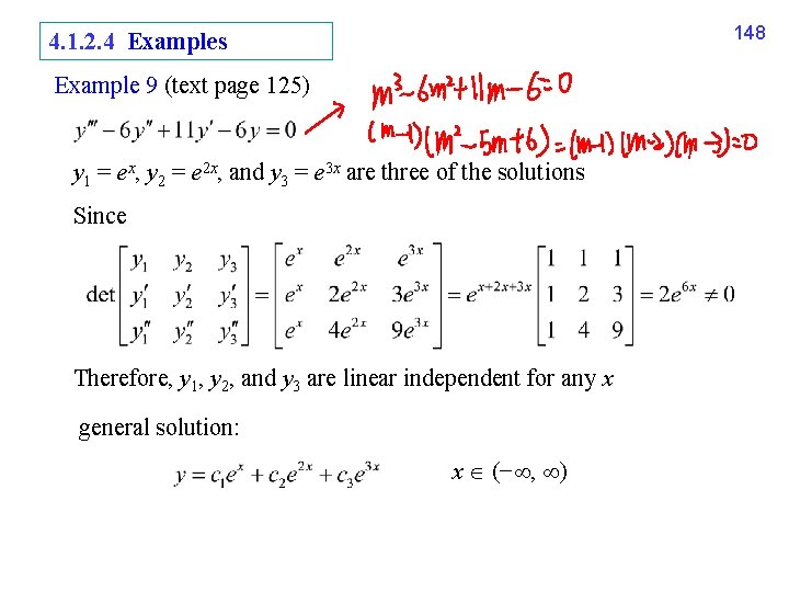
148 4. 1. 2. 4 Examples Example 9 (text page 125) y 1 = ex, y 2 = e 2 x, and y 3 = e 3 x are three of the solutions Since Therefore, y 1, y 2, and y 3 are linear independent for any x general solution: x (− , )

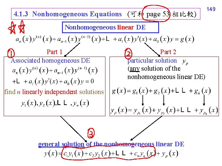
4. 1. 3 Nonhomogeneous Equations (可和 page 53 相比較) Nonhomogeneous linear DE Part 1 Associated homogeneous DE Part 2 particular solution (any solution of the nonhomogeneous linear DE) find n linearly independent solutions general solution of the nonhomogeneous linear DE 149

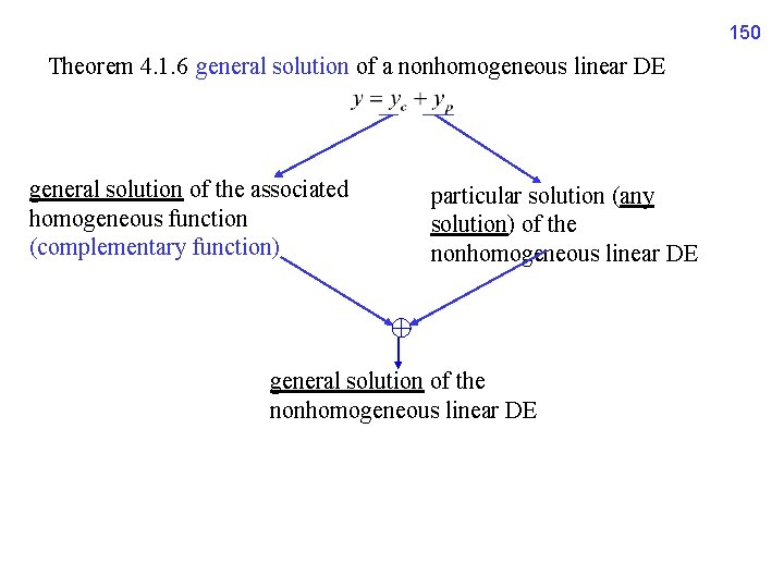
150 Theorem 4. 1. 6 general solution of a nonhomogeneous linear DE general solution of the associated homogeneous function (complementary function) particular solution (any solution) of the nonhomogeneous linear DE general solution of the nonhomogeneous linear DE

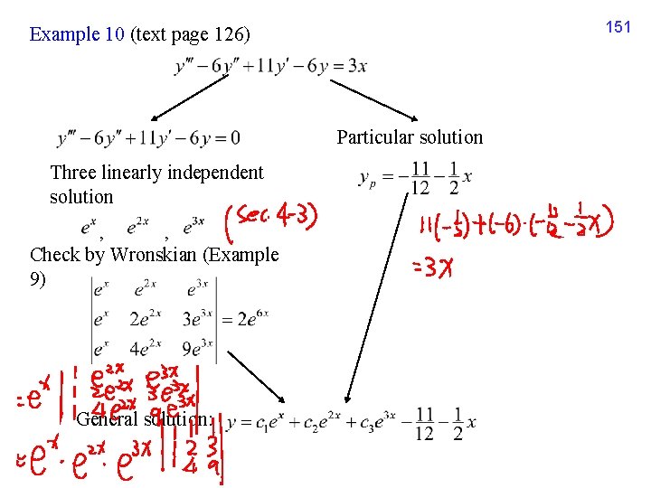
151 Example 10 (text page 126) Particular solution Three linearly independent solution , Check by Wronskian (Example 9) General solution:

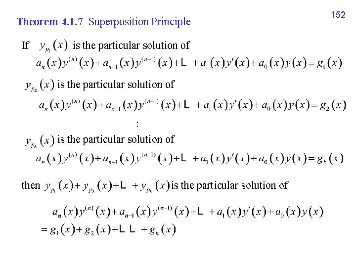
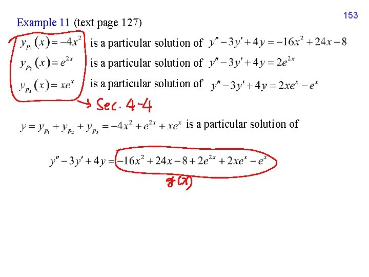
Theorem 4. 1. 7 Superposition Principle If is the particular solution of : is the particular solution of then is the particular solution of 152

Example 11 (text page 127) is a particular solution of is a particular solution of 153

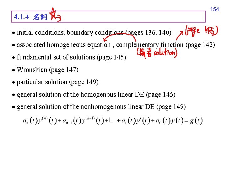
154 4. 1. 4 名詞 initial conditions, boundary conditions (pages 136, 140) associated homogeneous equation , complementary function (page 142) fundamental set of solutions (page 145) Wronskian (page 147) particular solution (page 149) general solution of the homogenous linear DE (page 145) general solution of the nonhomogenous linear DE (page 149)

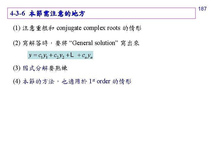
155 4. 1. 5 本節要注意的地方 (1) Most of theories in Section 4. 1 are applied to the linear DE (2) 注意 initial conditions 和 boundary conditions 之間的不同 (3) 快速判斷 linear independent

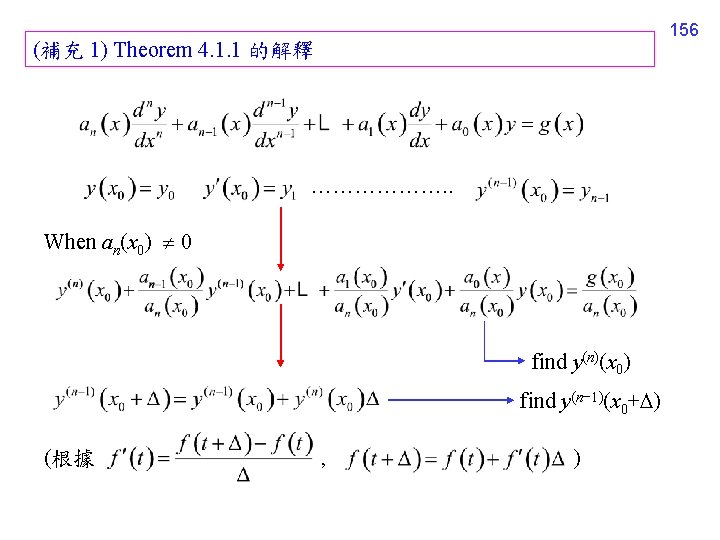
156 (補充 1) Theorem 4. 1. 1 的解釋 ………………. . When an(x 0) 0 find y(n)(x 0) find y(n− 1)(x 0+ ) (根據 , )

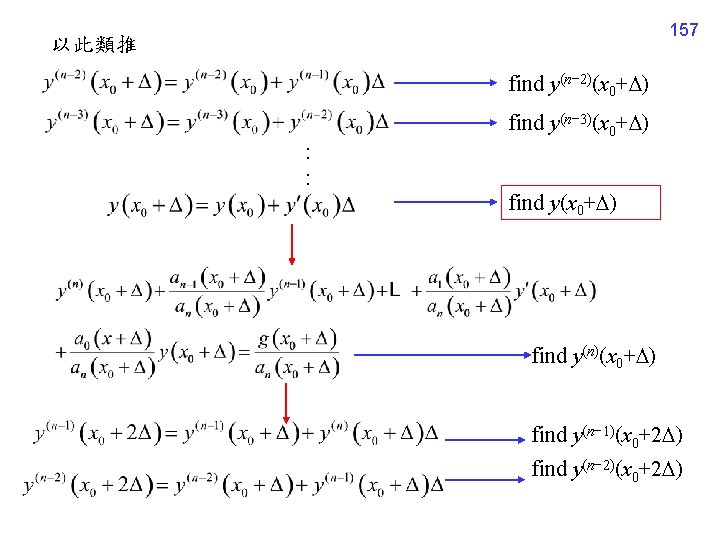
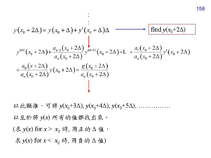
157 以此類推 find y(n− 2)(x 0+ ) find y(n− 3)(x 0+ ) : : find y(x 0+ ) find y(n)(x 0+ ) find y(n− 1)(x 0+2 ) find y(n− 2)(x 0+2 )

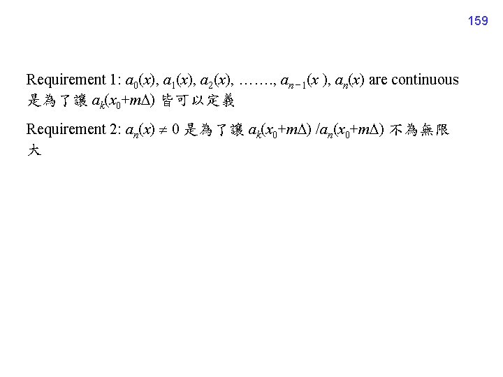
159 Requirement 1: a 0(x), a 1(x), a 2(x), ……. , an − 1(x ), an(x) are continuous 是為了讓 ak(x 0+m ) 皆可以定義 Requirement 2: an(x) 0 是為了讓 ak(x 0+m ) /an(x 0+m ) 不為無限 大

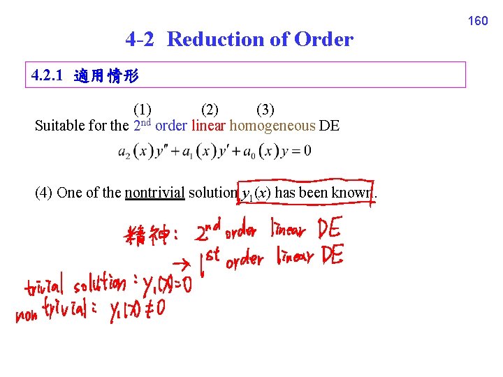
4 -2 Reduction of Order 4. 2. 1 適用情形 (1) (2) (3) Suitable for the 2 nd order linear homogeneous DE (4) One of the nontrivial solution y 1(x) has been known. 160

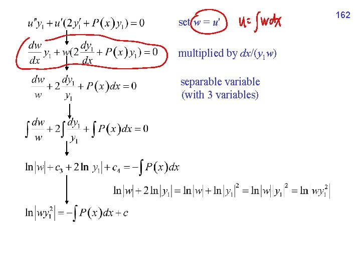
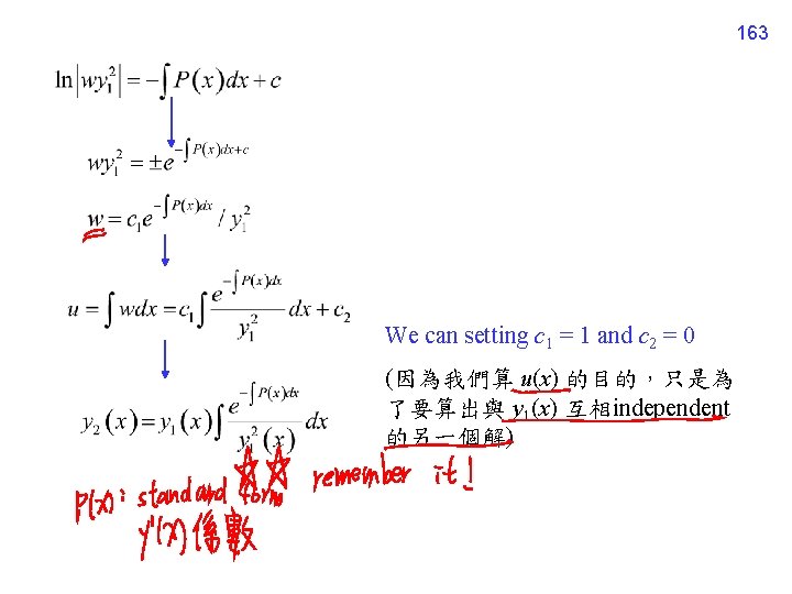
4. 2. 2 解法 假設 先將DE 變成 Standard form If y(x) = u(x) y 1(x) , zero 161

set w = u' multiplied by dx/(y 1 w) separable variable (with 3 variables) 162

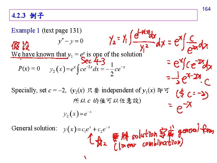
4. 2. 3 例子 Example 1 (text page 131) We have known that y 1 = ex is one of the solution P(x) = 0 Specially, set c = – 2, (y 2(x) 只要 independent of y 1(x) 即可 所以 c 的值可以任意設) General solution: 164

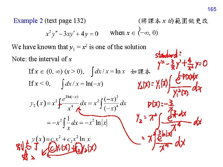
165 Example 2 (text page 132) (將課本 x 的範圍做更改 ) when x (− , 0) We have known that y 1 = x 2 is one of the solution Note: the interval of x If x (0, ) (x > 0), 如課本 If x < 0,

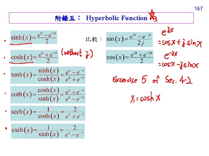
167 附錄五： Hyperbolic Function 比較：

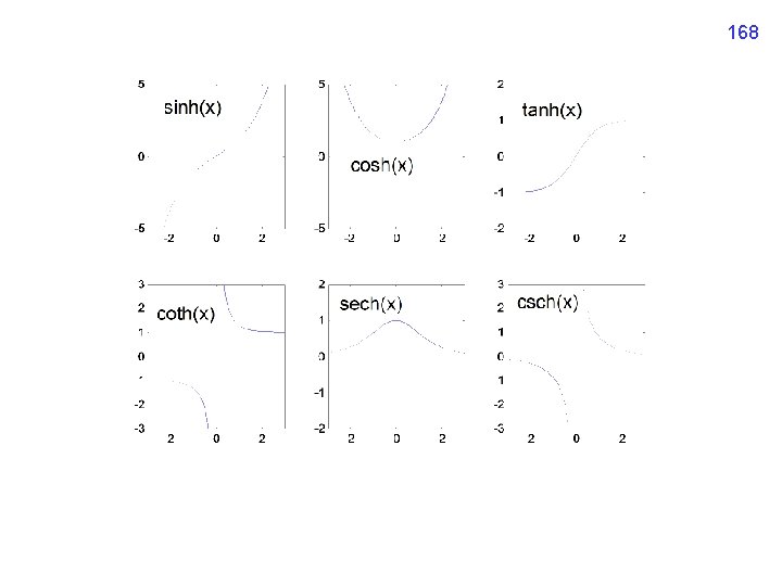
168

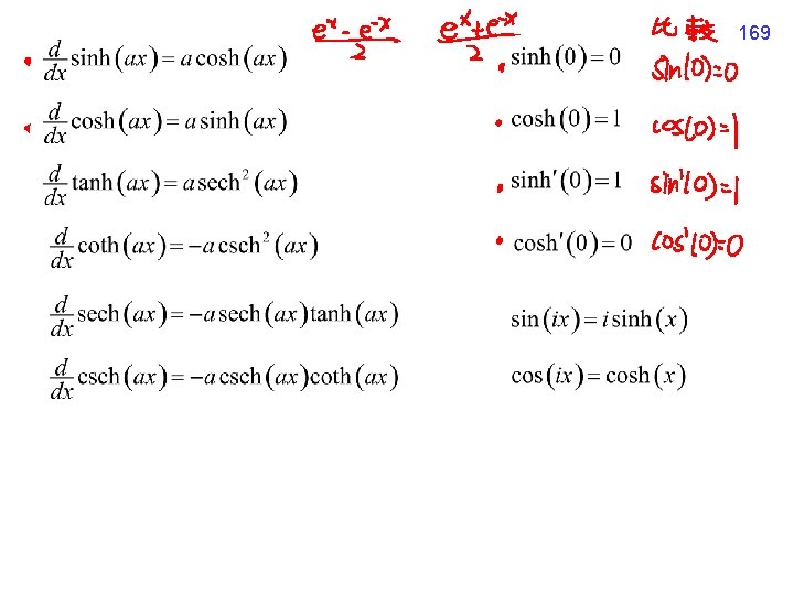
169

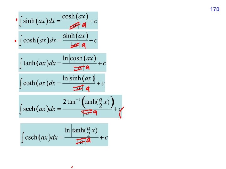
170

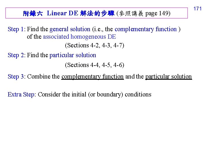
附錄六 Linear DE 解法的步驟 (參照講義 page 149) 171 Step 1: Find the general solution (i. e. , the complementary function ) of the associated homogeneous DE (Sections 4 -2, 4 -3, 4 -7) Step 2: Find the particular solution (Sections 4 -4, 4 -5, 4 -6) Step 3: Combine the complementary function and the particular solution Extra Step: Consider the initial (or boundary) conditions

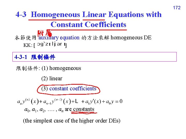
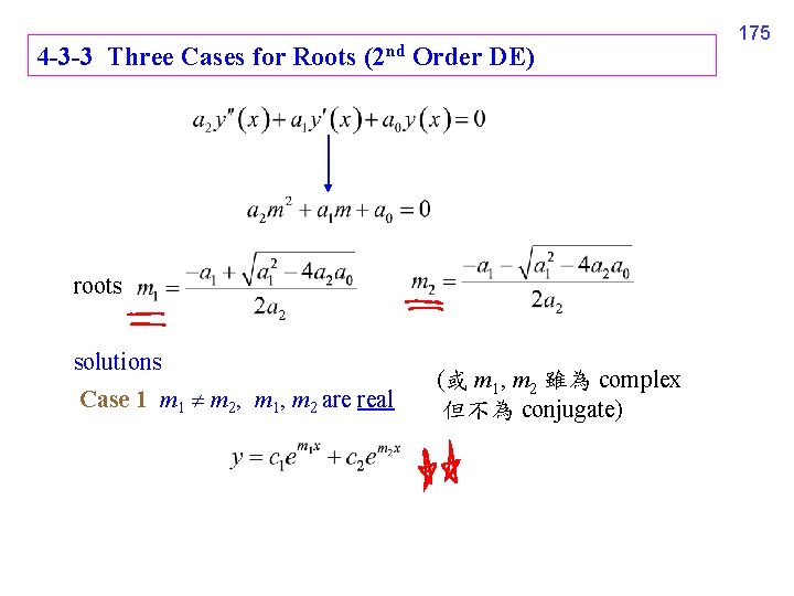
4 -3 Homogeneous Linear Equations with Constant Coefficients 本節使用 auxiliary equation 的方法來解 homogeneous DE KK: [ ] 4 -3 -1 限制條件: (1) homogeneous (2) linear (3) constant coefficients a 0, a 1, a 2, …. , an are constants (the simplest case of the higher order DEs) 172

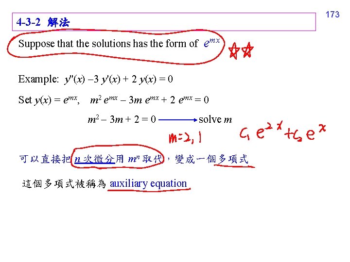
4 -3 -2 解法 Suppose that the solutions has the form of emx Example: y''(x) 3 y'(x) + 2 y(x) = 0 Set y(x) = emx, m 2 emx 3 m emx + 2 emx = 0 m 2 3 m + 2 = 0 solve m 可以直接把 n 次微分用 mn 取代，變成一個多項式 這個多項式被稱為 auxiliary equation 173

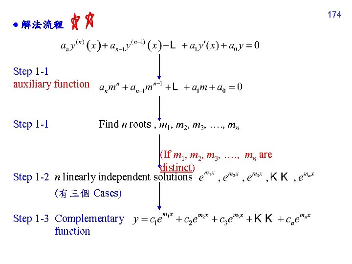
174 解法流程 Step 1 -1 auxiliary function Step 1 -1 Find n roots , m 1, m 2, m 3, …. , mn (If m 1, m 2, m 3, …. , mn are distinct) Step 1 -2 n linearly independent solutions (有三個 Cases) Step 1 -3 Complementary function

4 -3 -3 Three Cases for Roots (2 nd Order DE) roots solutions Case 1 m 1 m 2, m 1, m 2 are real (或 m 1, m 2 雖為 complex 但不為 conjugate) 175

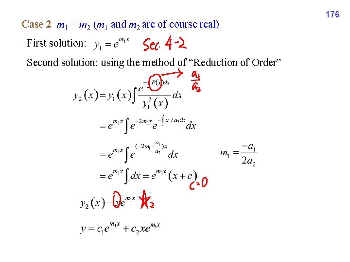
Case 2 m 1 = m 2 (m 1 and m 2 are of course real) First solution: Second solution: using the method of “Reduction of Order” 176

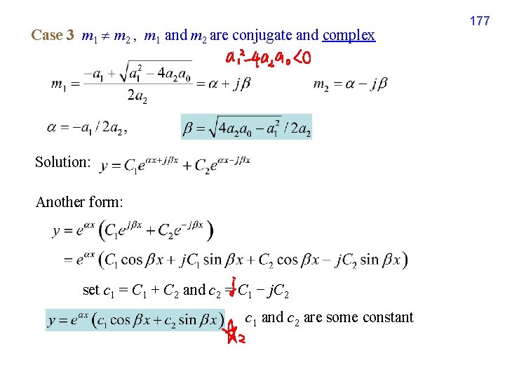
Case 3 m 1 m 2 , m 1 and m 2 are conjugate and complex Solution: Another form: set c 1 = C 1 + C 2 and c 2 = C 1 − j. C 2 c 1 and c 2 are some constant 177

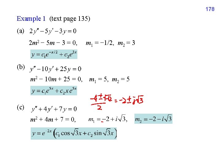
178 Example 1 (text page 135) (a) 2 m 2 − 5 m − 3 = 0, m 1 = − 1/2, m 2 = 3 (b) m 2 − 10 m + 25 = 0, m 1 = 5, m 2 = 5 (c) m 2 + 4 m + 7 = 0,

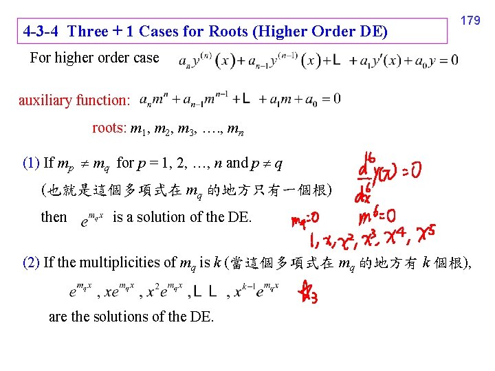
4 -3 -4 Three + 1 Cases for Roots (Higher Order DE) 179 For higher order case auxiliary function: roots: m 1, m 2, m 3, …. , mn (1) If mp mq for p = 1, 2, …, n and p q (也就是這個多項式在 mq 的地方只有一個根) then is a solution of the DE. (2) If the multiplicities of mq is k (當這個多項式在 mq 的地方有 k 個根), are the solutions of the DE.

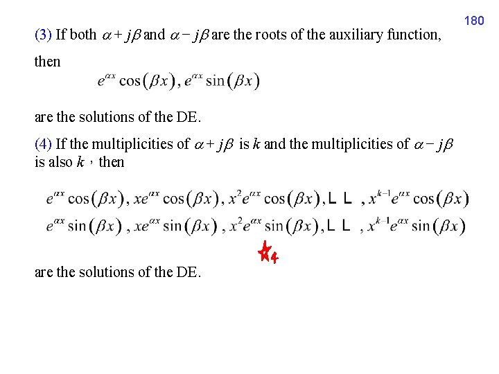
(3) If both + j and − j are the roots of the auxiliary function, then are the solutions of the DE. (4) If the multiplicities of + j is k and the multiplicities of − j is also k，then are the solutions of the DE. 180

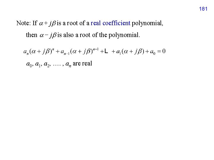
181 Note: If + j is a root of a real coefficient polynomial, then − j is also a root of the polynomial. a 0, a 1, a 2, …. , an are real

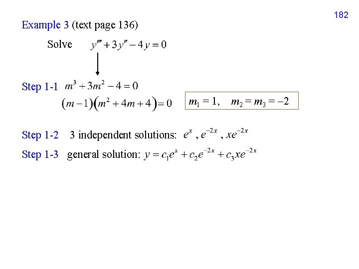
182 Example 3 (text page 136) Solve Step 1 -1 m 1 = 1, m 2 = m 3 = 2 Step 1 -2 3 independent solutions: Step 1 -3 general solution:

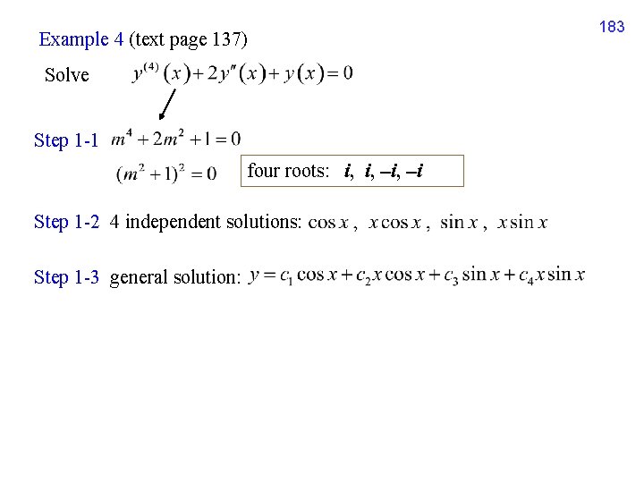
Example 4 (text page 137) Solve Step 1 -1 four roots: i, i, i Step 1 -2 4 independent solutions: Step 1 -3 general solution: 183

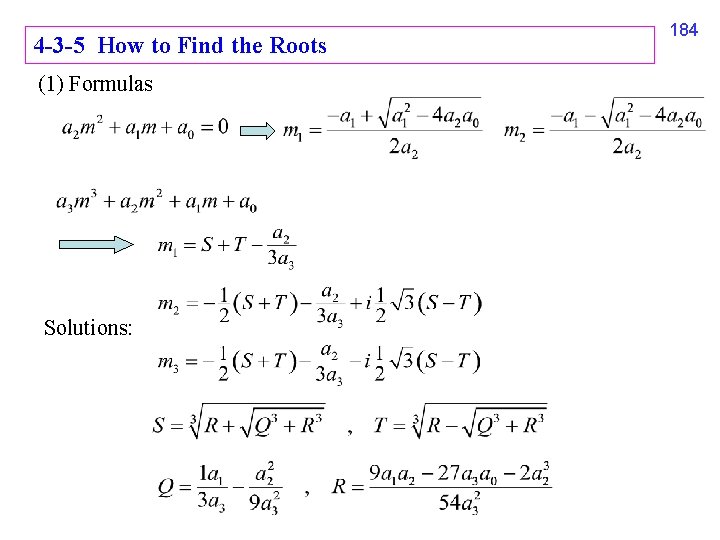
4 -3 -5 How to Find the Roots (1) Formulas Solutions: 184

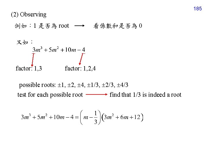
185 (2) Observing 例如： 1 是否為 root 看係數和是否為 0 又如： factor: 1, 3 factor: 1, 2, 4 possible roots: 1, 2, 4, 1/3, 2/3, 4/3 test for each possible root find that 1/3 is indeed a root

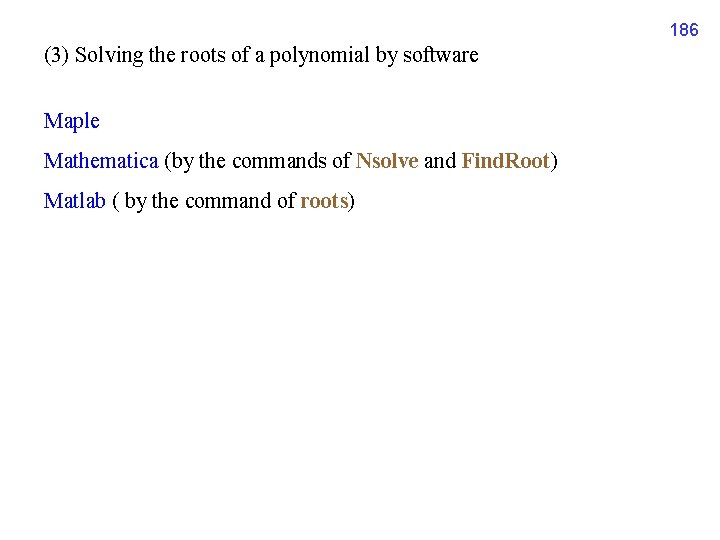
186 (3) Solving the roots of a polynomial by software Maple Mathematica (by the commands of Nsolve and Find. Root) Matlab ( by the command of roots)

188 Exercise for practice Sec. 4 -1: 3, 7, 8, 13, 20, 24, 29, 33, 36 Sec. 4 -2: 2, 4, 9, 13, 14, 18, 19 Sec. 4 -3: 7, 16, 20, 24, 28, 33, 39, 41, 50, 51

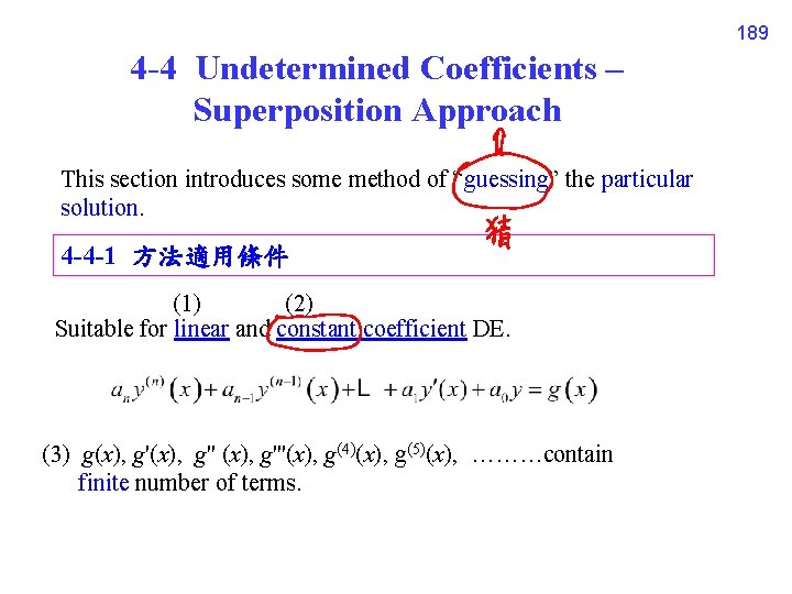
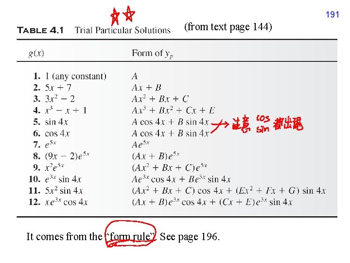
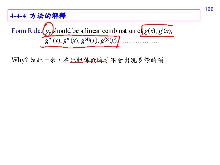
189 4 -4 Undetermined Coefficients – Superposition Approach This section introduces some method of “guessing” the particular solution. 4 -4 -1 方法適用條件 (1) (2) Suitable for linear and constant coefficient DE. (3) g(x), g'(x), g'' (x), g'''(x), g(4)(x), g(5)(x), ………contain finite number of terms.

191 (from text page 144) It comes from the “form rule”. See page 196.

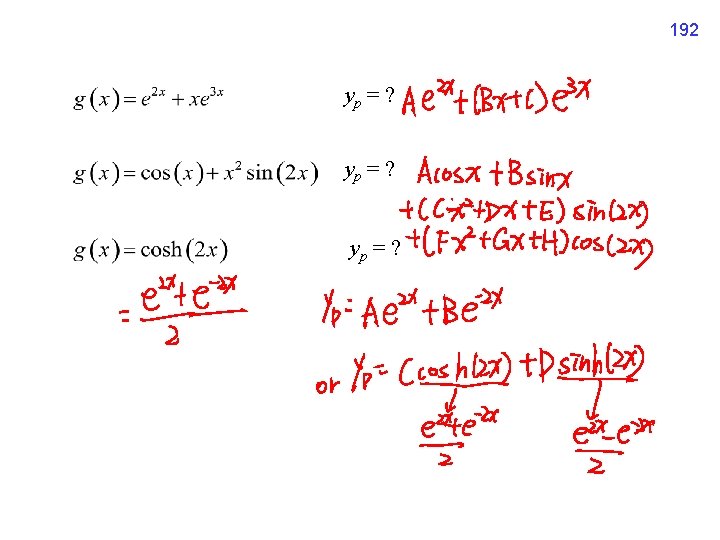
192 yp = ?

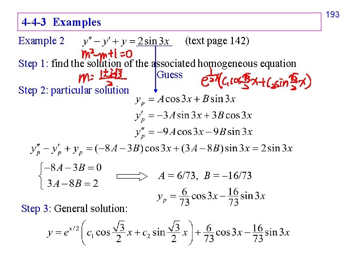
193 4 -4 -3 Examples Example 2 (text page 142) Step 1: find the solution of the associated homogeneous equation Guess Step 2: particular solution A = 6/73, B = 16/73 Step 3: General solution:

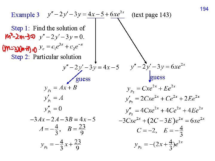
Example 3 (text page 143) Step 1: Find the solution of Step 2: Particular solution guess 194

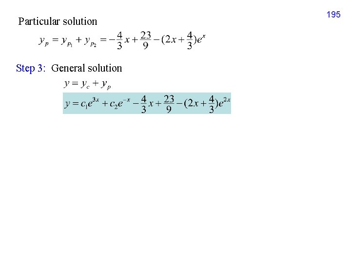
Particular solution Step 3: General solution 195

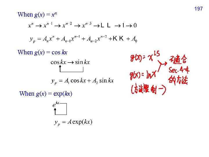
When g(x) = xn When g(x) = cos kx When g(x) = exp(kx) 197

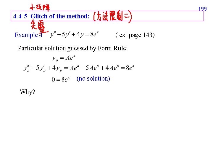
199 4 -4 -5 Glitch of the method: Example 4 (text page 143) Particular solution guessed by Form Rule: (no solution) Why?

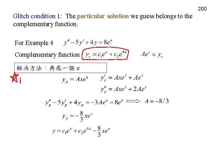
200 Glitch condition 1: The particular solution we guess belongs to the complementary function. For Example 4 Complementary function 解決方法：再乘一個 x

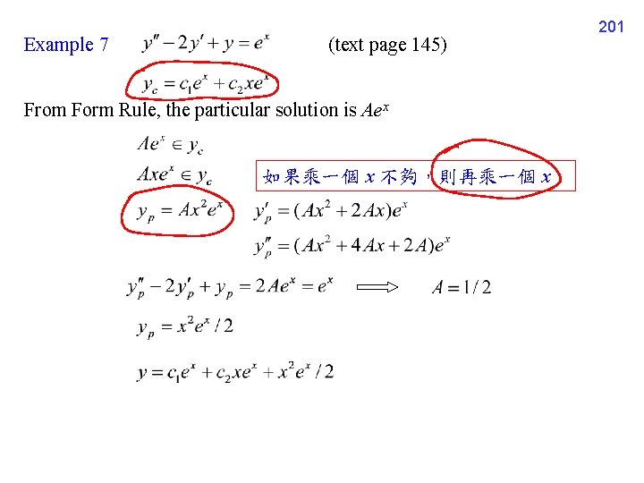
Example 7 (text page 145) From Form Rule, the particular solution is Aex 如果乘一個 x 不夠，則再乘一個 x 201

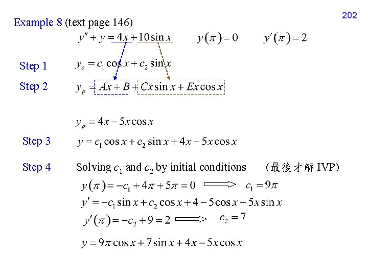
202 Example 8 (text page 146) Step 1 Step 2 Step 3 Step 4 Solving c 1 and c 2 by initial conditions (最後才解 IVP)

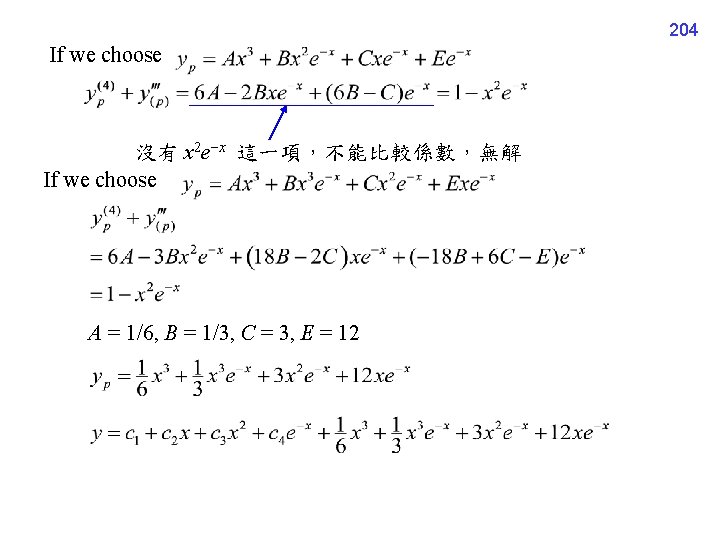
204 If we choose 沒有 x 2 e x 這一項，不能比較係數，無解 If we choose A = 1/6, B = 1/3, C = 3, E = 12

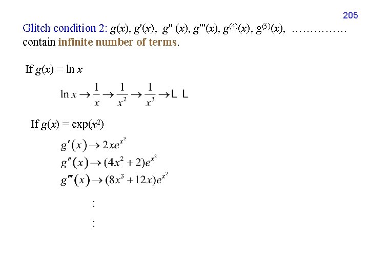
205 Glitch condition 2: g(x), g'(x), g'' (x), g'''(x), g(4)(x), g(5)(x), …………… contain infinite number of terms. If g(x) = ln x If g(x) = exp(x 2) : :

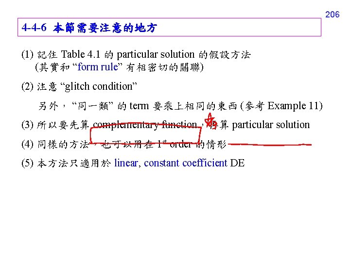
206 4 -4 -6 本節需要注意的地方 (1) 記住 Table 4. 1 的 particular solution 的假設方法 (其實和 “form rule” 有相密切的關聯) (2) 注意 “glitch condition” 另外， “同一類” 的 term 要乘上相同的東西 (參考 Example 11) (3) 所以要先算 complementary function，再算 particular solution (4) 同樣的方法，也可以用在 1 st order 的情形 (5) 本方法只適用於 linear, constant coefficient DE