50 th Anniversary of The Curse of Dimensionality

50 th Anniversary of The Curse of Dimensionality • Continuous States: Storage cost: resolutiondx Computational cost: resolutiondx • Continuous Actions: Computational cost: resolutiondu

Beating The Curse Of Dimensionality • • • Reduce dimensionality (biped examples) Use primitives (Poincare section) Parameterize V, policy (future lecture) Reduce volume of state space explored Use greater depth search Adaptive/Problem-specific grid/sampling – Split where needed – Random sampling – add where needed • Random action search • Random state search • Hybrid Approaches: combine local and global opt.

Use Brute Force • Deal with computational cost by using cluster supercomputer. • Main issue is minimizing communication between nodes.

Cluster Supercomputing • • (8) Cores w/ small local memory (cache) (100) Nodes w/ shared memory (16 GB) (4 -16 Gb/s) Network (100 T) Disks

Q(x, u) = L(x, u) + V(f(x, u)) • c = L(x, u): as in desktop case • x_next = f(x, u): as in desktop case • V(x_next) – Uniform grid – Multilinear interpolation if all values available, distance weighted averaging if bad values

Allocate grid to cores/nodes

Handle Overlap

Push Updated V’s To Users

So what does this all mean for programming? • On a node, split grid cells among threads, which execute on cores. • Share updates of V(x) and u(x) within node almost for free using shared memory. • Pushing updated V(x) and u(x) to other nodes uses the network which is relatively slow…. .

Dealing with the slow network • Organize grid cells into packet-sized blocks. Send them as a unit. • Threshold updates: too small, don’t send it. • Only do 1/N updates for each block (maximum skip time). • Tolerate packet loss (UDP) vs. verification (TCP/MPI)

Use Adaptive Grid • Reduce computational and storage costs by using adaptive grid. • Generate adaptive grid using random sampling.

Trajectory-Based Dynamic Programming

Full Trajectories Helps Reduce Resolution Needed SIDP Trajectory Based

Reducing the Volume Explored

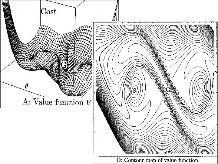
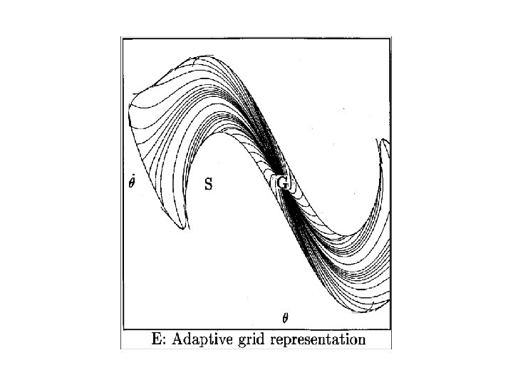
An Adaptive Grid Approach

Global Planning Propagate Value Function Across Trajectories in Adaptive Grid

Growing the Explored Region: Adaptive Grids

Bidirectional Search

Bidirectional Search Closeup

Spine Representation

Growing the Explored Region: Spine Representation

Comparison

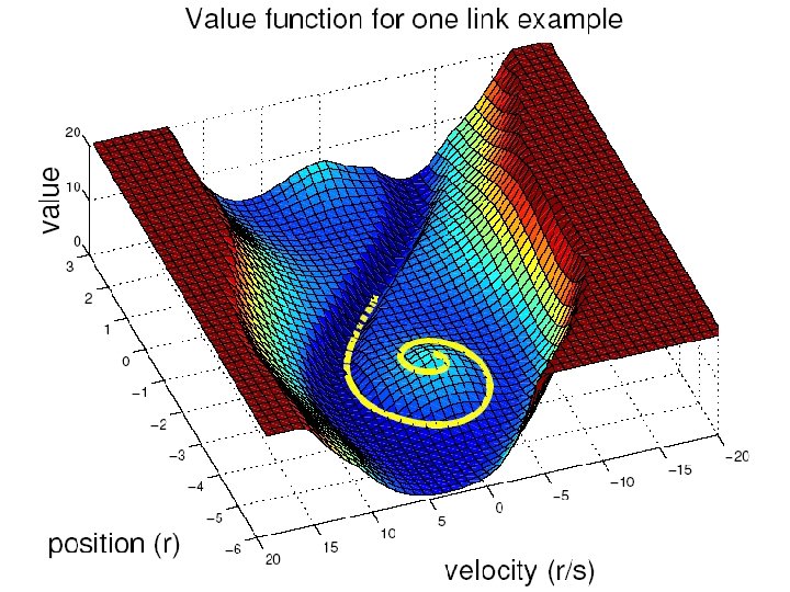
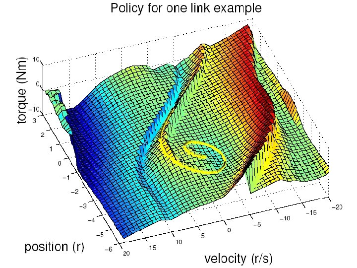
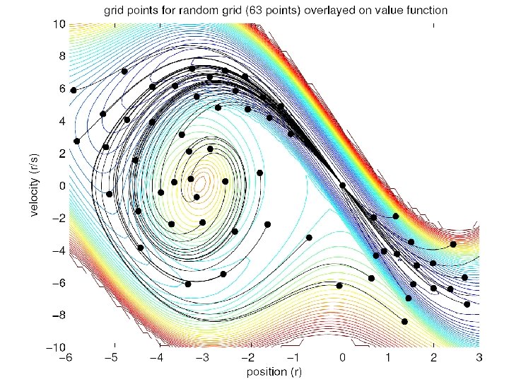
One Link Swing Up Needed Only 63 Points

Trajectories For Each Point

Random Sampling of States • Initialize with a point at the goal with local models based on LQR. • Choose a random new state x. • Use the nearest stored point’s local model of the value function to predict the value of the new point (VP). • Optimize a trajectory from x to the goal. At each step use the nearest stored point’s local model of the policy to create an action. Use DDP to refine this trajectory. VT is cost of trajectory starting from x. • Store point at start of trajectory if |VT - VP |> λ (surprise), VT < Vlimit and VP < Vlimit, otherwise discard. • Interleave re-optimization of all stored points. Only update if Vnew < V (V is upper bound on value). • Gradually increase Vlimit.

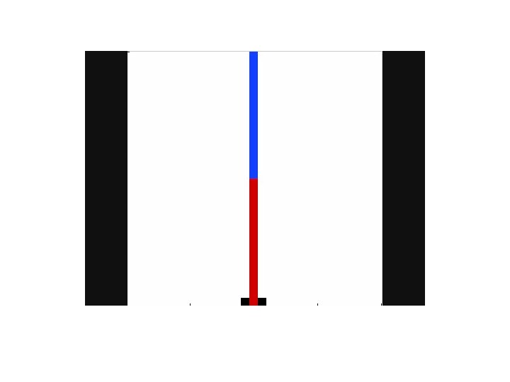
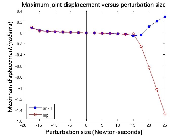
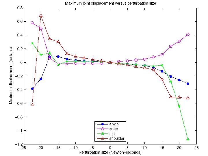
Two Link Pendulum • Criterion:

Ankle Angle Ankle Torque Hip Angle Hip Torque

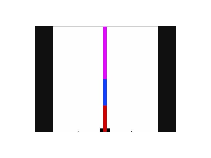
Four Links

Four Links: 8 dimensional system

Convergence? • Because we create trajectories to the goal, each value function estimate at a point is an upper bound for the value at that point. • Eventually all value function entries will be consistent with their nearest neighbor’s local model, and no new points can be added. • We are using more aggressive acceptance tests for new points: VB < λVP, λ < 1, and VP < Vlimit vs. |VB – VP| < ε and VB < Vlimit • Not clear if needed new points can be blocked.

Use Local Models • Try to achieve a sparse representation using local models.

Linear Quadratic Regulators

Learning From Observation

Regulator tasks • Examples: balance a pole, move at a constant velocity • A reasonable starting point is a Linear Quadratic Regulator (LQR controller) • Might have nonlinear dynamics xk+1 = f(xk, uk), but since stay around xd, can locally linearize xk+1 = Axk + Buk • Might have complex scoring function c(x, u), but can locally approximate with a quadratic model c x. TQx + u. TRu • dlqr() in matlab

Linearization Example • • • Iθdd = -mgl sin(θ) – μθd + τ Linearize Discretize time Vectorize (θ θd) k+1 T = (1 T; -mgl. T/I 1 -μT/I) (θ θd) k. T + (0 T/I)T τk

LQR Derivation • • Assume V() quadratic: Vk+1(x) = x. TVxx: k+1 x C(x, u) = x. TQx + u. TRu + (Ax+Bu)TVxx: k+1 (Ax+Bu) Want C/ u = 0 BTVxx: k+1 Ax = -(BTVxx: k+1 B + R)u u = Kx (linear controller) K = - (BTVxx: k+1 B + R)-1 BTVxx: k+1 A Vxx: k= ATVxx: k+1 A + Q + ATVxx: k+1 BK

Trajectory Optimization (closed loop) • Differential Dynamic Programming (local approach to DP).

Learning Trajectories

Q function • • x: state, u: control or action Dynamics: xk+1 = f(xk, uk) Cost function: L(x, u) Value function V(x) = ∑L(x, u) Q function Q(x, u) = L(x, u) + V(f(x, u)) Bellman’s Equation V(x) = minu Q(x, u) Policy/control law: u(x) = argminu Q(x, u)

Local Models About

Propagating Local Models Along a Trajectory: Differential Dynamic Programming Gradient version • Vx: k-1 = Qx = Lx + Vxfx • Δu = Qu = Lu + Vxfu

Differential Dynamic Programming (DDP) [Mc. Reynolds 70, Jacobson 70] Value function (update) Execution Improved trajectory Terminal V(T) Initial Require: • Dynamics model • Penalty function Nominal trajectory Q(T-2) u’(T-2) V(T-2) Q(T-1): Action value function u’(T-1): New control output V(T-1): State value function t

Propagating Local Models Along a Trajectory: Differential Dynamic Programming

Levenberg Marquardt • • • y = f(x) minx (s = y. Ty/2) gradient ∂s/∂x = (∂f/∂x)Ty = JTy Hessian ∂2 s/∂2 x = H = (∂2 f/∂2 x) y + JTJ 2 nd order gradient descent Δx = H-1 JTy Problem: H not positive definite Solution: Δx = (H + λI)-1 JTy λ small: 2 nd order approach λ large: 1 st order approach, Δx = JTy/λ Trick 2: H ≈ JTJ

Levenberg Marquardt-like DDP • Δu = (Quu + λI)-1 Qu • K = (Quu + λI)-1 Qux • Drop fxx, fxu, fux, and fuu terms

Other tricks • If Δu fails, try ε Δu • Just optimize last part of trajectory. • Regularize Qxx

Neighboring Optimal Control

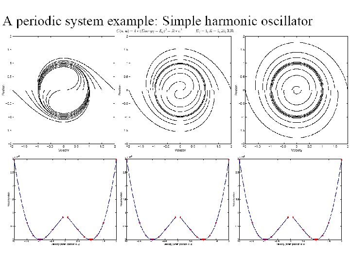
What Changes When Task Periodic? • Discount factor means V() might increase along trajectory. V() cannot always decrease in periodic tasks.

Robot Hopper Example

Dimensionality Reduction • Use of simple models (for example LIPM) • Poincaré section

Inverted Pendulum Model • Massless legs • State: pitch angular velocity at TOP • Controls: ankle torque, step length ø

Optimization Criterion • T is step duration; Ta is ankle torque; ø is leg swing angle; Vd is desired velocity. • Ankle torque: ∑(Ta 2) • Swing leg acceleration: (ø/T 2)2 • Match desired velocity: (2 sin(ø/2)/T – Vd)2 • Criterion is weighted sum of above terms.

Poincaré Section Transition Top Poincaré section

Optimal Controller For Sagittal Plane Only (Vd=1) Foot Placement Policy Ankle Torque Policy Return Map Value Function VELOCITY

Return Map (Vd=1)

Optimal Controller For Sagittal Plane Only (Vd=1) Foot Placement Policy Ankle Torque Policy Return Map Value Function VELOCITY

Foot Placement Policies

Ankle Torque Policies

Return Maps

Add Torso ø h ø

Optimization Criteria • Ankle torque: ∑(Ta 2) • Swing leg acceleration: (ø/T 2)2 • Match desired velocity: (2 sin(ø/2)/T – Vd)2 • Desired torso angle: ∑(ψd)2

Simulation

Simulation

Commands

Torso

What difference does a torso make?

3 D version: Add roll • State: pitch velocity, roll velocity at TOP • Action 1: Sagittal foot placement • Action 2: Sagittal ankle torque • Action 3: Lateral foot placement

Roll Optimization Criteria • T = step duration. • Ankle torque: torque 2 • Swing leg acceleration: (ø/T 2)2 • Match desired velocity: (2 sin(ø/2)/T – Vd)2 • Roll leg acceleration: (øroll/T 2)2

Lateral foot placement at fixed roll