Dimensionality reduction Why dimensionality reduction n Some features

Dimensionality reduction

Why dimensionality reduction? n Some features may be irrelevant n We want to visualize high dimensional data n “Intrinsic” dimensionality may be smaller than the number of features

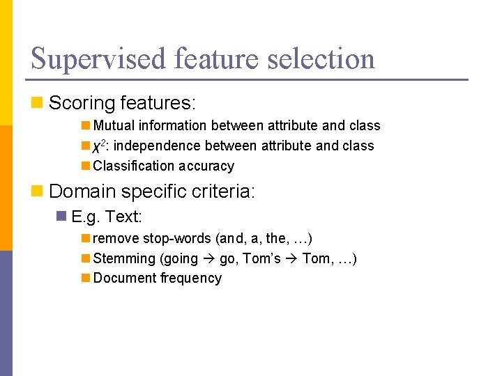
Supervised feature selection n Scoring features: n Mutual information between attribute and class n χ2: independence between attribute and class n Classification accuracy n Domain specific criteria: n E. g. Text: n remove stop-words (and, a, the, …) n Stemming (going go, Tom’s Tom, …) n Document frequency

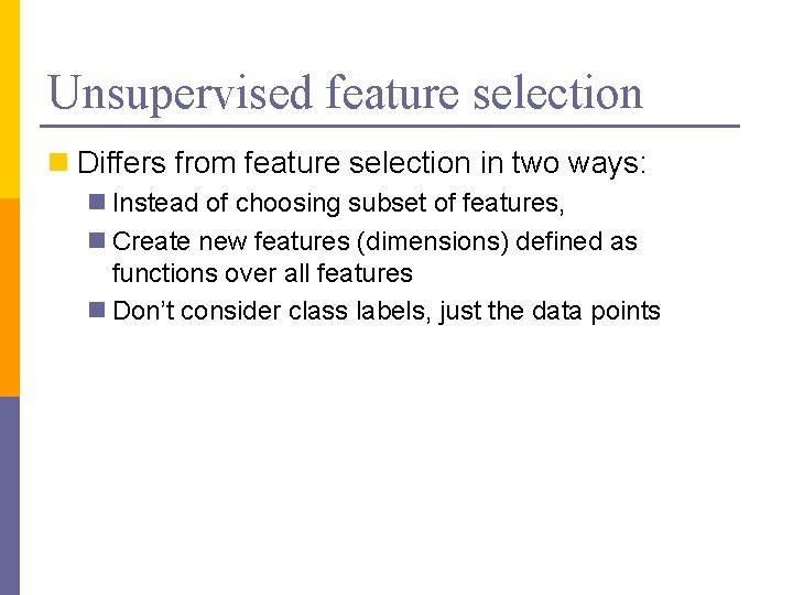
Unsupervised feature selection n Differs from feature selection in two ways: n Instead of choosing subset of features, n Create new features (dimensions) defined as functions over all features n Don’t consider class labels, just the data points

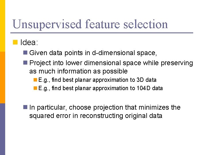
Unsupervised feature selection n Idea: n Given data points in d-dimensional space, n Project into lower dimensional space while preserving as much information as possible n E. g. , find best planar approximation to 3 D data n E. g. , find best planar approximation to 104 D data n In particular, choose projection that minimizes the squared error in reconstructing original data

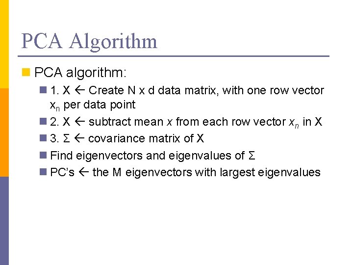
PCA Algorithm n PCA algorithm: n 1. X Create N x d data matrix, with one row vector xn per data point n 2. X subtract mean x from each row vector xn in X n 3. Σ covariance matrix of X n Find eigenvectors and eigenvalues of Σ n PC’s the M eigenvectors with largest eigenvalues

2 d Data

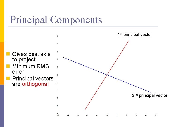
Principal Components 1 st principal vector n Gives best axis to project n Minimum RMS error n Principal vectors are orthogonal 2 nd principal vector

How many components? n Check the distribution of eigen-values n Take enough eigen-vectors to cover 80 -90% of the variance

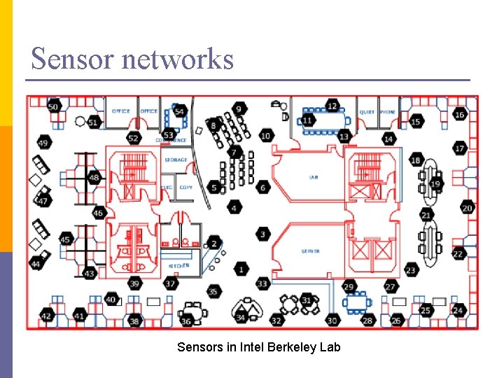
Sensor networks Sensors in Intel Berkeley Lab

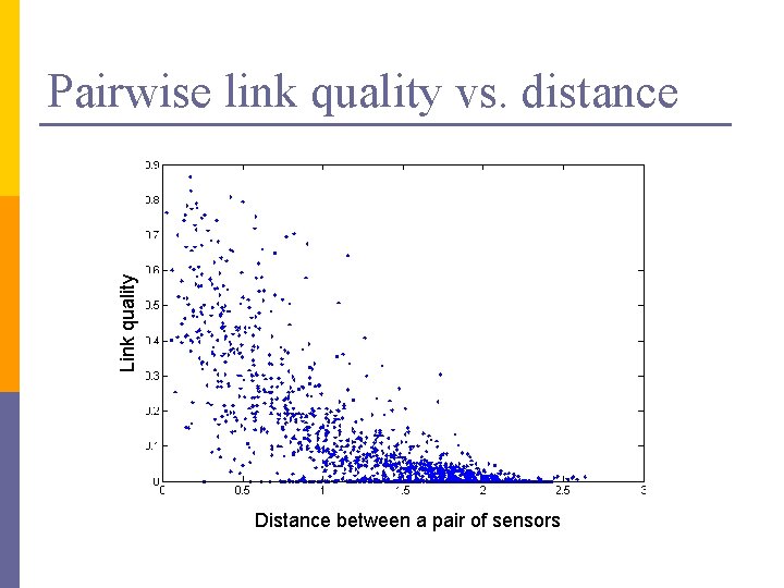
Link quality Pairwise link quality vs. distance Distance between a pair of sensors

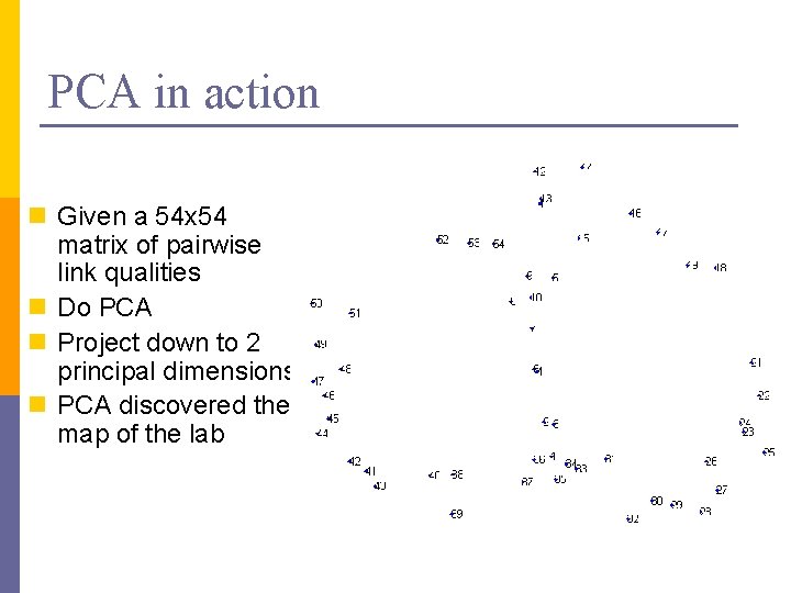
PCA in action n Given a 54 x 54 matrix of pairwise link qualities n Do PCA n Project down to 2 principal dimensions n PCA discovered the map of the lab

Problems and limitations n What if very large dimensional data? n e. g. , Images (d ≥ 104) n Problem: n Covariance matrix Σ is size (d 2) n d=104 |Σ| = 108 n Singular Value Decomposition (SVD)! n efficient algorithms available (Matlab) n some implementations find just top N eigenvectors

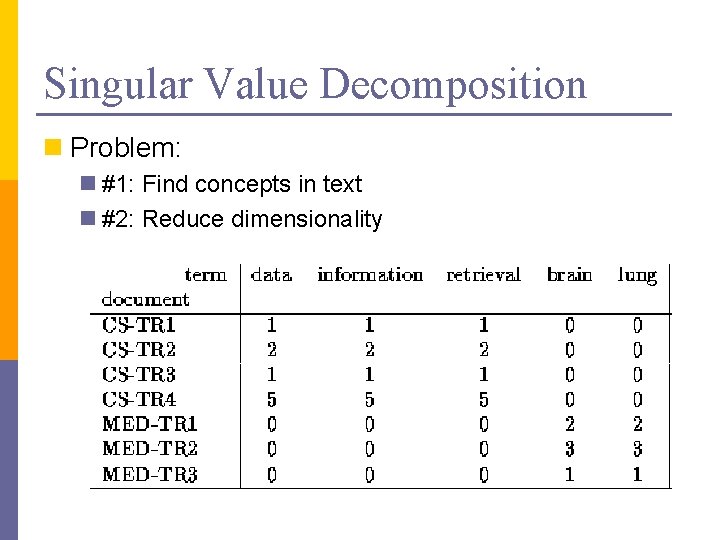
Singular Value Decomposition n Problem: n #1: Find concepts in text n #2: Reduce dimensionality

SVD - Definition A[n x m] = U[n x r] L [ r x r] (V[m x r])T n A: n x m matrix (e. g. , n documents, m terms) n U: n x r matrix (n documents, r concepts) n L: r x r diagonal matrix (strength of each ‘concept’) (r: rank of the matrix) n V: m x r matrix (m terms, r concepts)

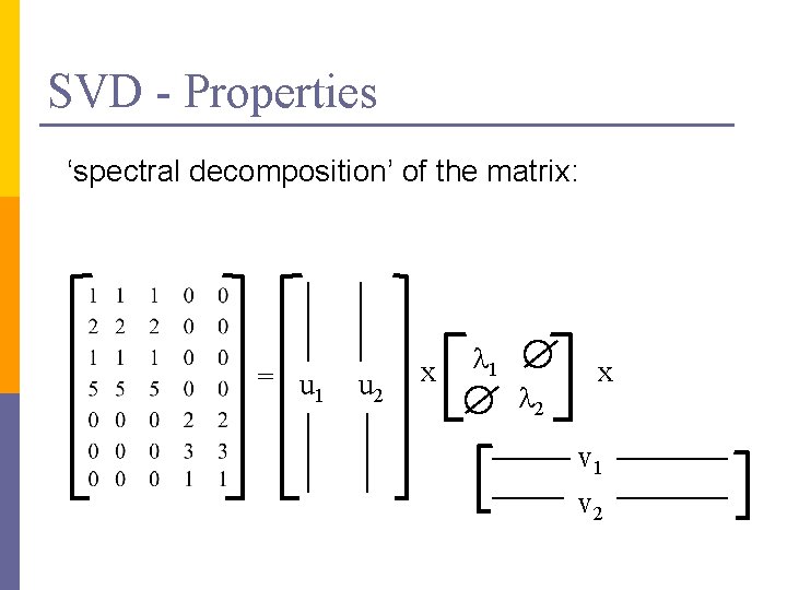
SVD - Properties THEOREM [Press+92]: always possible to decompose matrix A into A = U L VT , where n U, L, V: unique n U, V: column orthonormal (ie. , columns are unit vectors, orthogonal to each other) n UTU = I; VTV = I (I: identity matrix) n L: singular value are positive, and sorted in decreasing order

SVD - Properties ‘spectral decomposition’ of the matrix: = u 1 u 2 x l 1 l 2 x v 1 v 2

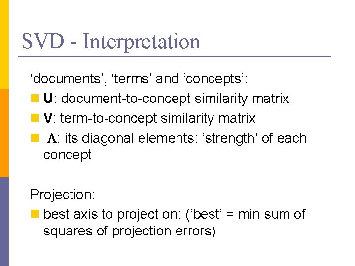
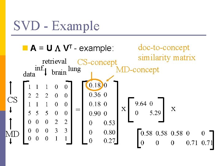
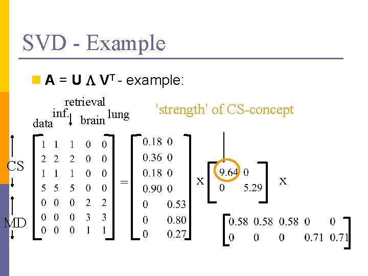
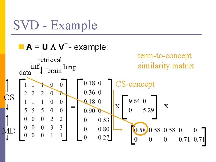
SVD - Interpretation ‘documents’, ‘terms’ and ‘concepts’: n U: document-to-concept similarity matrix n V: term-to-concept similarity matrix n L: its diagonal elements: ‘strength’ of each concept Projection: n best axis to project on: (‘best’ = min sum of squares of projection errors)

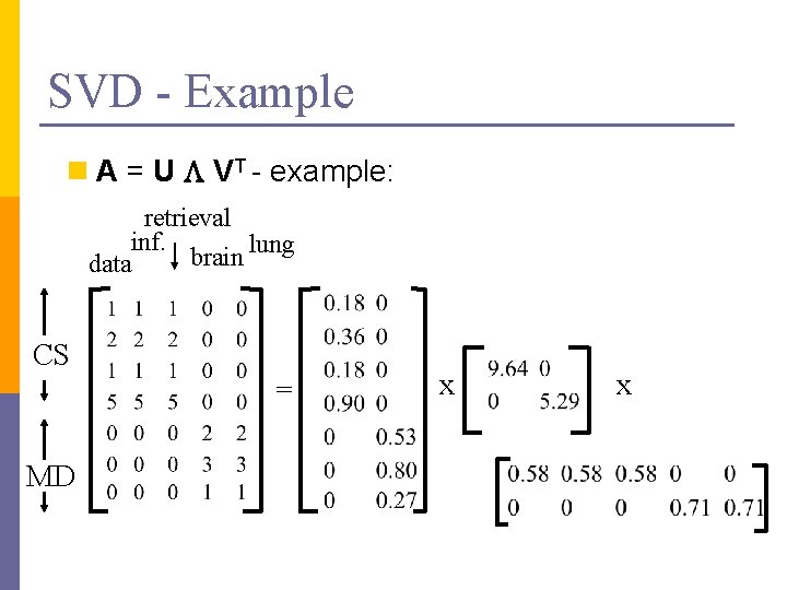
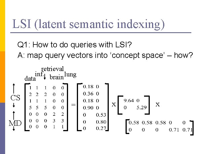
SVD - Example n A = U L VT - example: retrieval inf. lung brain data CS = MD x x

SVD - Example doc-to-concept similarity matrix retrieval CS-concept inf. MD-concept brain lung n A = U L VT - example: data CS = MD x x

SVD - Example n A = U L VT - example: retrieval inf. lung brain data CS = MD ‘strength’ of CS-concept x x

SVD - Example n A = U L VT - example: term-to-concept similarity matrix retrieval inf. lung brain data CS-concept CS = MD x x

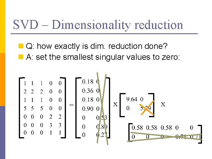
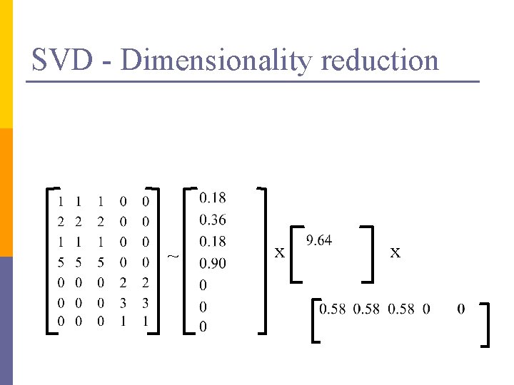
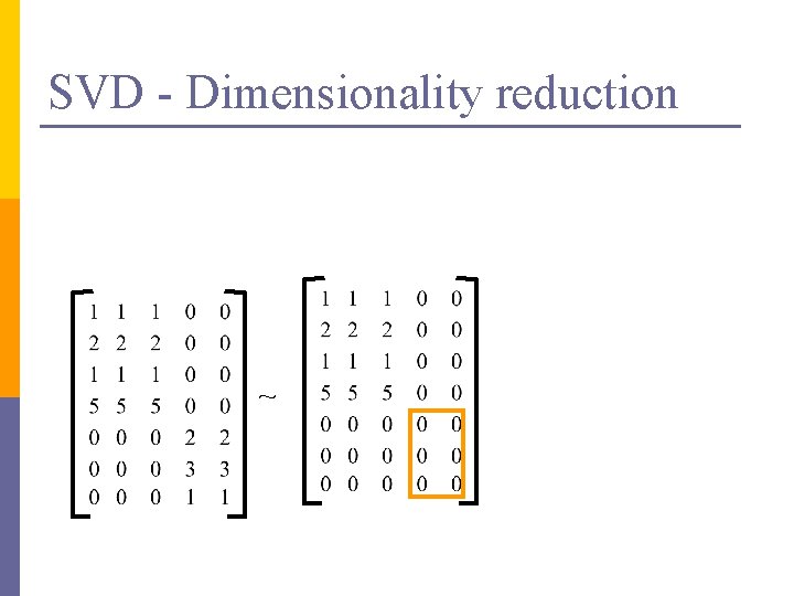
SVD – Dimensionality reduction n Q: how exactly is dim. reduction done? n A: set the smallest singular values to zero: = x x

SVD - Dimensionality reduction ~ x x

SVD - Dimensionality reduction ~

LSI (latent semantic indexing) Q 1: How to do queries with LSI? A: map query vectors into ‘concept space’ – how? retrieval inf. brain lung data CS MD = x x

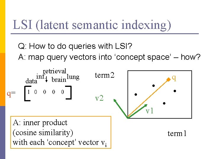
LSI (latent semantic indexing) Q: How to do queries with LSI? A: map query vectors into ‘concept space’ – how? retrieval inf. brain lung data q= term 2 q v 2 v 1 A: inner product (cosine similarity) with each ‘concept’ vector vi term 1

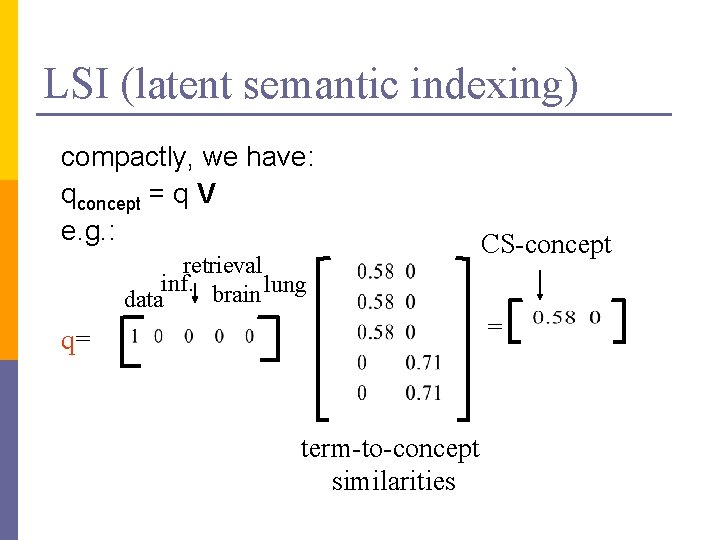
LSI (latent semantic indexing) compactly, we have: qconcept = q V e. g. : retrieval inf. brain lung data q= term-to-concept similarities CS-concept =

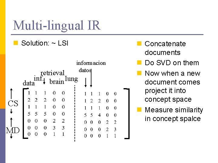
Multi-lingual IR (English query, on Spanish text? ) Q: multi-lingual IR (english query, on spanish text? ) n Problem: n given many documents, translated to both languages (eg. , English and Spanish) n answer queries across languages

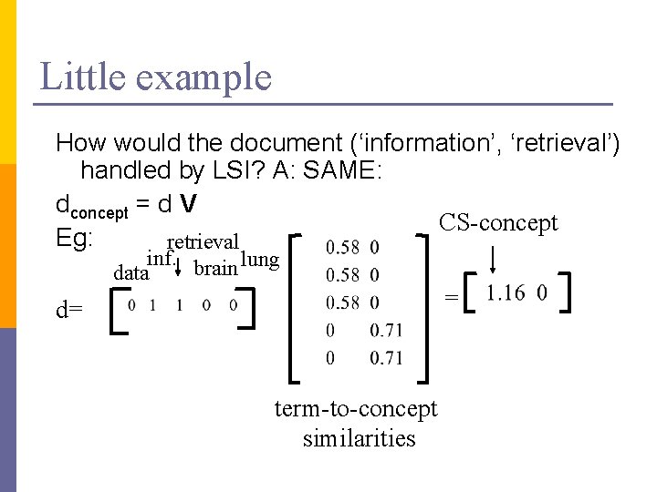
Little example How would the document (‘information’, ‘retrieval’) handled by LSI? A: SAME: dconcept = d V CS-concept Eg: retrieval inf. brain lung data = d= term-to-concept similarities

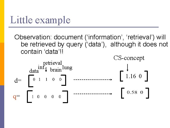
Little example Observation: document (‘information’, ‘retrieval’) will be retrieved by query (‘data’), although it does not contain ‘data’!! CS-concept retrieval inf. brain lung data d= q=

Multi-lingual IR n Solution: ~ LSI informacion datos retrieval inf. brain lung data CS MD n Concatenate documents n Do SVD on them n Now when a new document comes project it into concept space n Measure similarity in concept spalce

Visualization of text n Given a set of documents how could we visualize them over time? n Idea: n Perform PCA n Project documents down to 2 dimensions n See how the cluster centers change – observe the words in the cluster over time

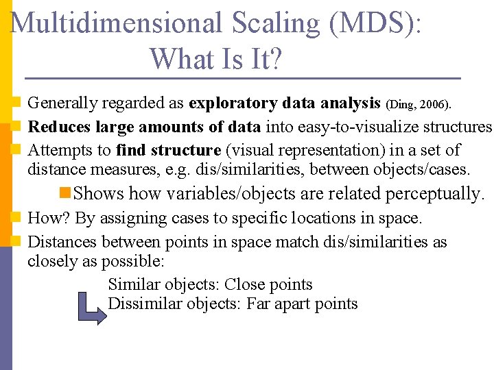
Multidimensional Scaling (MDS): What Is It? n Generally regarded as exploratory data analysis (Ding, 2006). n Reduces large amounts of data into easy-to-visualize structures. n Attempts to find structure (visual representation) in a set of distance measures, e. g. dis/similarities, between objects/cases. n. Shows how variables/objects are related perceptually. n How? By assigning cases to specific locations in space. n Distances between points in space match dis/similarities as closely as possible: Similar objects: Close points Dissimilar objects: Far apart points

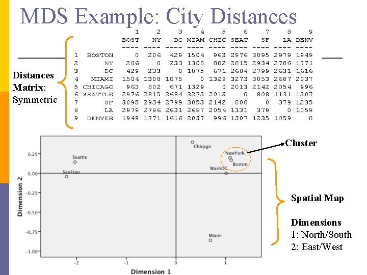
MDS Example: City Distances Matrix: Symmetric Cluster Spatial Map Dimensions 1: North/South 2: East/West

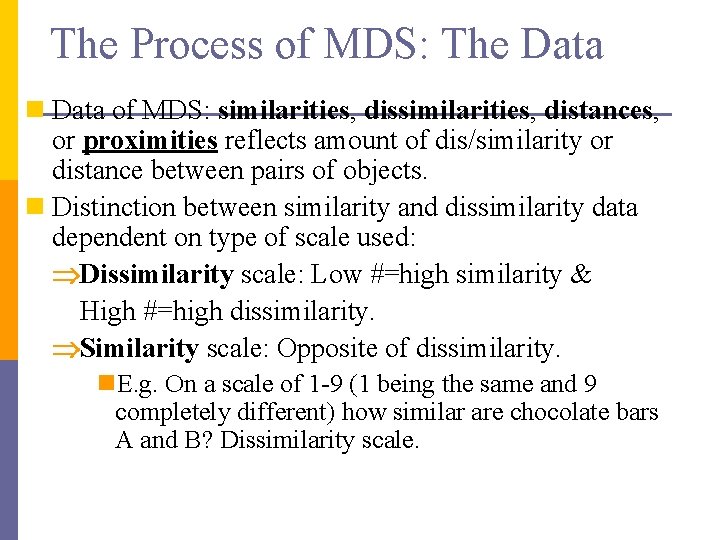
The Process of MDS: The Data n Data of MDS: similarities, distances, or proximities reflects amount of dis/similarity or distance between pairs of objects. n Distinction between similarity and dissimilarity data dependent on type of scale used: Dissimilarity scale: Low #=high similarity & High #=high dissimilarity. Similarity scale: Opposite of dissimilarity. n. E. g. On a scale of 1 -9 (1 being the same and 9 completely different) how similar are chocolate bars A and B? Dissimilarity scale.

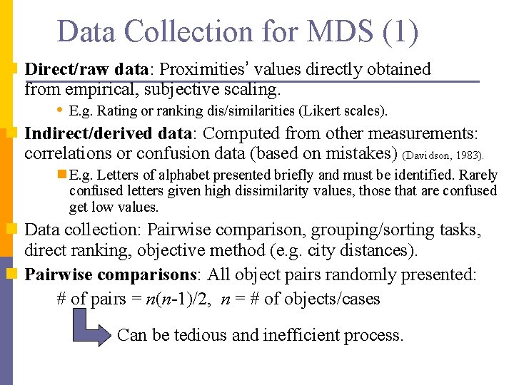
Data Collection for MDS (1) n Direct/raw data: Proximities’ values directly obtained from empirical, subjective scaling. • E. g. Rating or ranking dis/similarities (Likert scales). n Indirect/derived data: Computed from other measurements: correlations or confusion data (based on mistakes) (Davidson, 1983). n E. g. Letters of alphabet presented briefly and must be identified. Rarely confused letters given high dissimilarity values, those that are confused get low values. n Data collection: Pairwise comparison, grouping/sorting tasks, direct ranking, objective method (e. g. city distances). n Pairwise comparisons: All object pairs randomly presented: # of pairs = n(n-1)/2, n = # of objects/cases Can be tedious and inefficient process.

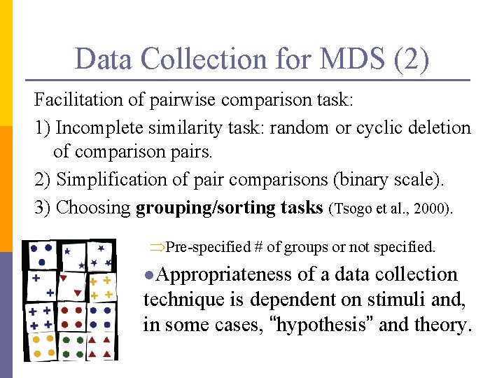
Data Collection for MDS (2) Facilitation of pairwise comparison task: 1) Incomplete similarity task: random or cyclic deletion of comparison pairs. 2) Simplification of pair comparisons (binary scale). 3) Choosing grouping/sorting tasks (Tsogo et al. , 2000). Pre-specified # of groups or not specified. l. Appropriateness of a data collection technique is dependent on stimuli and, in some cases, “hypothesis” and theory.

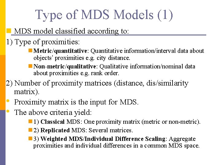
Type of MDS Models (1) n MDS model classified according to: 1) Type of proximities: n Metric/quantitative: Quantitative information/interval data about objects’ proximities e. g. city distance. n Non-metric/qualitative: Qualitative information/nominal data about proximities e. g. rank order. 2) Number of proximity matrices (distance, dis/similarity matrix). • Proximity matrix is the input for MDS. • The above criteria yield: n 1) Classical MDS: One proximity matrix (metric or non-metric). n 2) Replicated MDS: Several matrices. n 3) Weighted MDS/Individual Difference Scaling: Aggregate proximities and individual differences in a common MDS space.

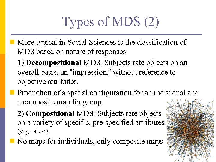
Types of MDS (2) n More typical in Social Sciences is the classification of MDS based on nature of responses: 1) Decompositional MDS: Subjects rate objects on an overall basis, an “impression, ” without reference to objective attributes. n Production of a spatial configuration for an individual and a composite map for group. 2) Compositional MDS: Subjects rate objects on a variety of specific, pre-specified attributes (e. g. size). n No maps for individuals, only composite maps.

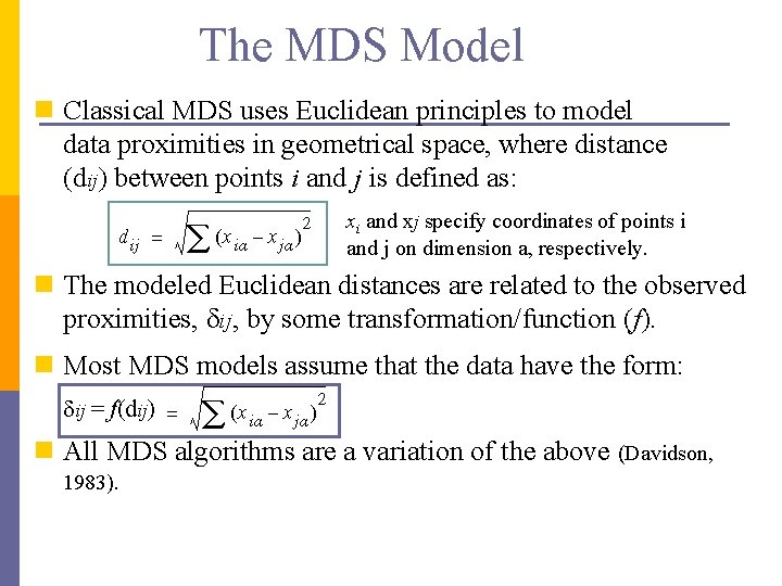
The MDS Model n Classical MDS uses Euclidean principles to model data proximities in geometrical space, where distance (dij) between points i and j is defined as: xi and xj specify coordinates of points i and j on dimension a, respectively. n The modeled Euclidean distances are related to the observed proximities, ij, by some transformation/function (f). n Most MDS models assume that the data have the form: ij = f(dij) n All MDS algorithms are a variation of the above (Davidson, 1983).

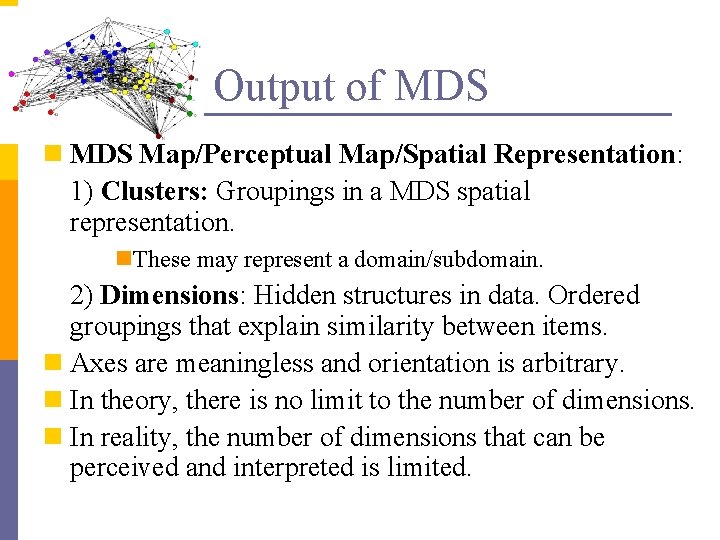
Output of MDS n MDS Map/Perceptual Map/Spatial Representation: 1) Clusters: Groupings in a MDS spatial representation. n. These may represent a domain/subdomain. 2) Dimensions: Hidden structures in data. Ordered groupings that explain similarity between items. n Axes are meaningless and orientation is arbitrary. n In theory, there is no limit to the number of dimensions. n In reality, the number of dimensions that can be perceived and interpreted is limited.

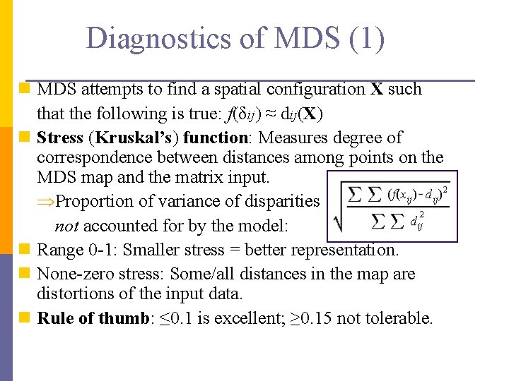
Diagnostics of MDS (1) n MDS attempts to find a spatial configuration X such that the following is true: f(δij) ≈ dij(X) n Stress (Kruskal’s) function: Measures degree of correspondence between distances among points on the MDS map and the matrix input. Proportion of variance of disparities not accounted for by the model: n Range 0 -1: Smaller stress = better representation. n None-zero stress: Some/all distances in the map are distortions of the input data. n Rule of thumb: ≤ 0. 1 is excellent; ≥ 0. 15 not tolerable.

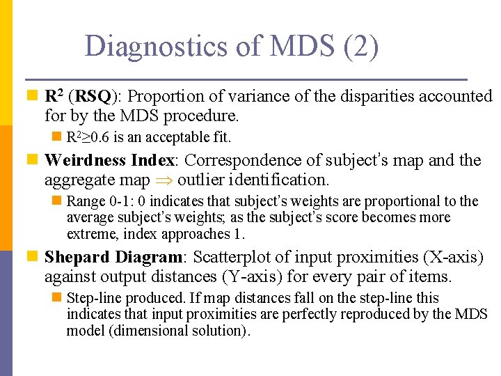
Diagnostics of MDS (2) n R 2 (RSQ): Proportion of variance of the disparities accounted for by the MDS procedure. n R 2≥ 0. 6 is an acceptable fit. n Weirdness Index: Correspondence of subject’s map and the aggregate map outlier identification. n Range 0 -1: 0 indicates that subject’s weights are proportional to the average subject’s weights; as the subject’s score becomes more extreme, index approaches 1. n Shepard Diagram: Scatterplot of input proximities (X-axis) against output distances (Y-axis) for every pair of items. n Step-line produced. If map distances fall on the step-line this indicates that input proximities are perfectly reproduced by the MDS model (dimensional solution).

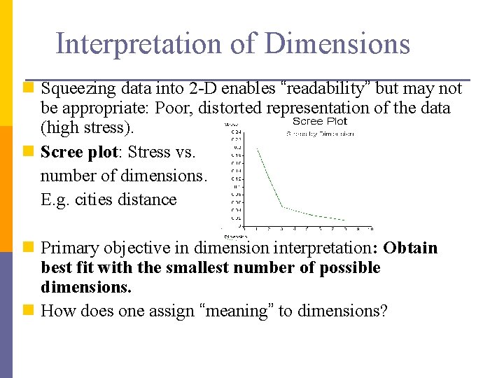
Interpretation of Dimensions n Squeezing data into 2 -D enables “readability” but may not be appropriate: Poor, distorted representation of the data (high stress). n Scree plot: Stress vs. number of dimensions. E. g. cities distance n Primary objective in dimension interpretation: Obtain best fit with the smallest number of possible dimensions. n How does one assign “meaning” to dimensions?

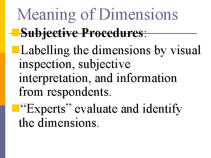
Meaning of Dimensions n. Subjective Procedures: n. Labelling the dimensions by visual inspection, subjective interpretation, and information from respondents. n“Experts” evaluate and identify the dimensions.

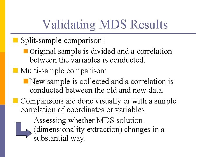
Validating MDS Results n Split-sample comparison: n Original sample is divided and a correlation between the variables is conducted. n Multi-sample comparison: n New sample is collected and a correlation is conducted between the old and new data. n Comparisons are done visually or with a simple correlation of coordinates or variables. Assessing whether MDS solution (dimensionality extraction) changes in a substantial way.

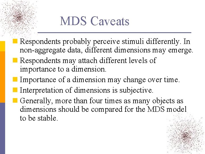
MDS Caveats n Respondents probably perceive stimuli differently. In non-aggregate data, different dimensions may emerge. n Respondents may attach different levels of importance to a dimension. n Importance of a dimension may change over time. n Interpretation of dimensions is subjective. n Generally, more than four times as many objects as dimensions should be compared for the MDS model to be stable.

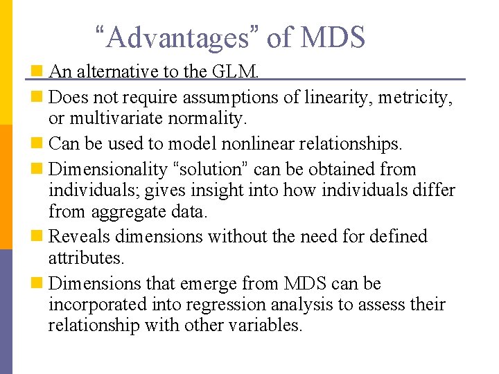
“Advantages” of MDS n An alternative to the GLM. n Does not require assumptions of linearity, metricity, or multivariate normality. n Can be used to model nonlinear relationships. n Dimensionality “solution” can be obtained from individuals; gives insight into how individuals differ from aggregate data. n Reveals dimensions without the need for defined attributes. n Dimensions that emerge from MDS can be incorporated into regression analysis to assess their relationship with other variables.

“Disadvantages” of MDS n Provides a global measure of dis/similarity but does not provide much insight into subtleties (Street et al. , 2001). n Increased dimensionality: Difficult to represent and decreases intuitive understanding of the data. As such, the model of the data becomes as complicated as the data itself. n Determination of meanings of dimensions is subjective.

A Tiny Break. . .

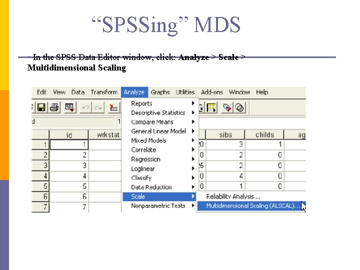
“SPSSing” MDS • In the SPSS Data Editor window, click: Analyze > Scale > Multidimensional Scaling

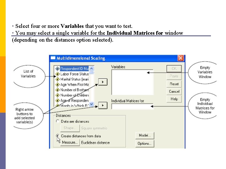
• Select four or more Variables that you want to test. • You may select a single variable for the Individual Matrices for window (depending on the distances option selected).

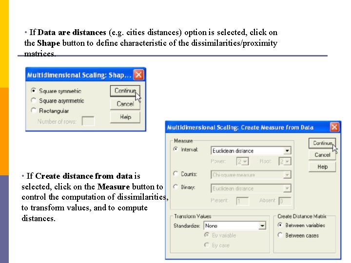
• If Data are distances (e. g. cities distances) option is selected, click on the Shape button to define characteristic of the dissimilarities/proximity matrices. • If Create distance from data is selected, click on the Measure button to control the computation of dissimilarities, to transform values, and to compute distances.

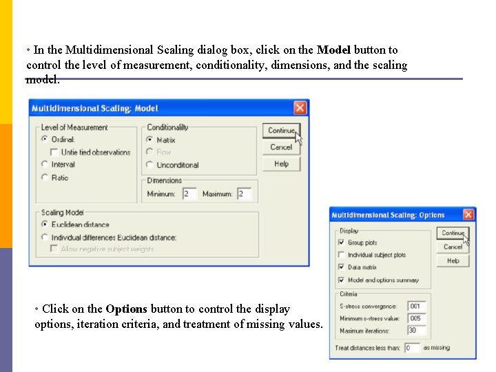
• In the Multidimensional Scaling dialog box, click on the Model button to control the level of measurement, conditionality, dimensions, and the scaling model. • Click on the Options button to control the display options, iteration criteria, and treatment of missing values.

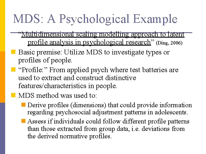
MDS: A Psychological Example “Multidimensional scaling modelling approach to latent profile analysis in psychological research” (Ding, 2006) n Basic premise: Utilize MDS to investigate types or profiles of people. n “Profile: ” From applied psych where test batteries are used to extract and construct distinctive features/characteristics in people. n MDS method was used to: n Derive profiles (dimensions) that could provide information regarding psychosocial adjustment patterns in adolescents. n Assess if individuals could follow different profile patterns than those extracted from group data, i. e. deviations from the derived normative profiles.

Study Details: Methodology n Participants: College students (µ=23 years, n=208). n Instruments: n Self-Image Questionnaire for Young Adolescents (SIQYA). Variables: n Body Image (BI), Peer Relationships (PR), Family Relationships (FR), Mastering & Coping (MC), Vocational-Educational Goals (VE), and Superior Adjustment (SA) n Three mental health measures of well-being: n Kandel Depression Scale n UCLA Loneliness Scale n Life Satisfaction Scale

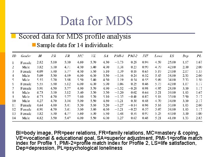
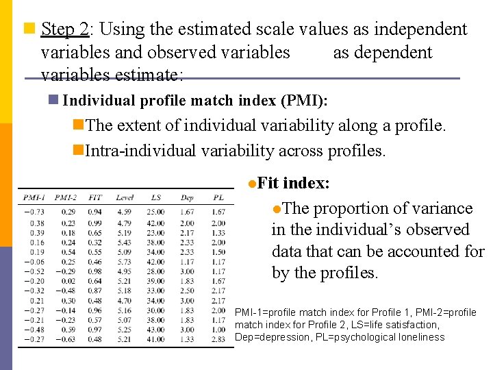
Data for MDS n Scored data for MDS profile analysis n Sample data for 14 individuals: BI=body image, PR=peer relations, FR=family relations, MC=mastery & coping, VE=vocational & educational goal, SA=superior adjustment, PMI-1=profile match index for Profile 1, PMI-2=profile match index for Profile 2, LS=life satisfaction, Dep=depression, PL=psychological loneliness

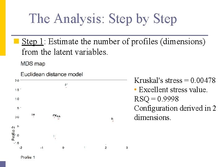
The Analysis: Step by Step n Step 1: Estimate the number of profiles (dimensions) from the latent variables. Kruskal's stress = 0. 00478 • Excellent stress value. RSQ = 0. 9998 Configuration derived in 2 dimensions.

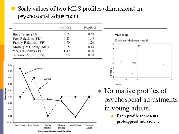
n Scale values of two MDS profiles (dimensions) in psychosocial adjustment. l Normative profiles of psychosocial adjustments in young adults. l Each profile represents prototypical individual.

n Step 2: Using the estimated scale values as independent variables and observed variables as dependent variables estimate: n Individual profile match index (PMI): n. The extent of individual variability along a profile. n. Intra-individual variability across profiles. l. Fit index: l. The proportion of variance in the individual’s observed data that can be accounted for by the profiles. PMI-1=profile match index for Profile 1, PMI-2=profile match index for Profile 2, LS=life satisfaction, Dep=depression, PL=psychological loneliness

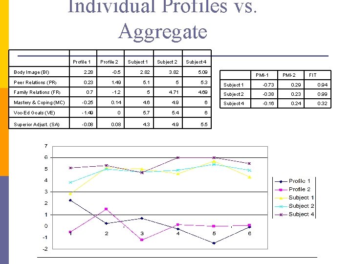
Individual Profiles vs. Aggregate Profile 1 Profile 2 Subject 1 Subject 2 Subject 4 Body Image (BI) 2. 28 -0. 5 2. 82 3. 82 5. 09 Peer Relations (PR) 0. 23 1. 49 5. 1 5 5. 3 Subject 1 -0. 73 0. 29 0. 94 0. 7 -1. 2 5 4. 71 4. 69 Subject 2 -0. 38 0. 23 0. 99 Mastery & Coping (MC) -0. 25 0. 14 4. 6 4. 9 6 Subject 4 -0. 16 0. 24 0. 32 Voc-Ed Goals (VE) -1. 49 0 5. 7 5. 4 6 Superior Adjust. (SA) -0. 08 4. 3 4. 9 5. 5 Family Relations (FR) PMI-1 PMI-2 FIT

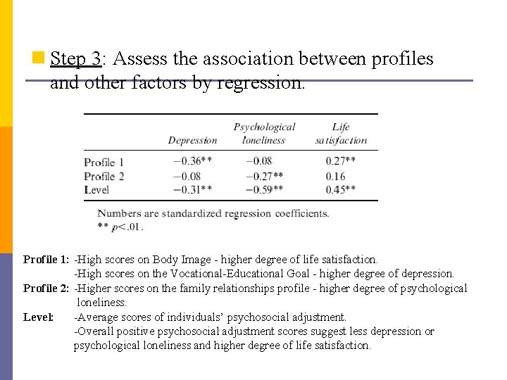
n Step 3: Assess the association between profiles and other factors by regression. Profile 1: -High scores on Body Image - higher degree of life satisfaction. -High scores on the Vocational-Educational Goal - higher degree of depression. Profile 2: -Higher scores on the family relationships profile - higher degree of psychological loneliness. Level: -Average scores of individuals’ psychosocial adjustment. -Overall positive psychosocial adjustment scores suggest less depression or psychological loneliness and higher degree of life satisfaction.

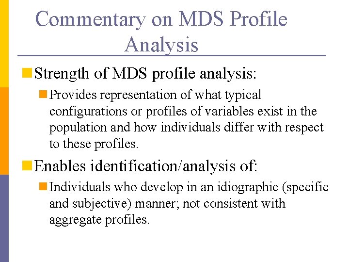
Commentary on MDS Profile Analysis n Strength of MDS profile analysis: n Provides representation of what typical configurations or profiles of variables exist in the population and how individuals differ with respect to these profiles. n Enables identification/analysis of: n Individuals who develop in an idiographic (specific and subjective) manner; not consistent with aggregate profiles.

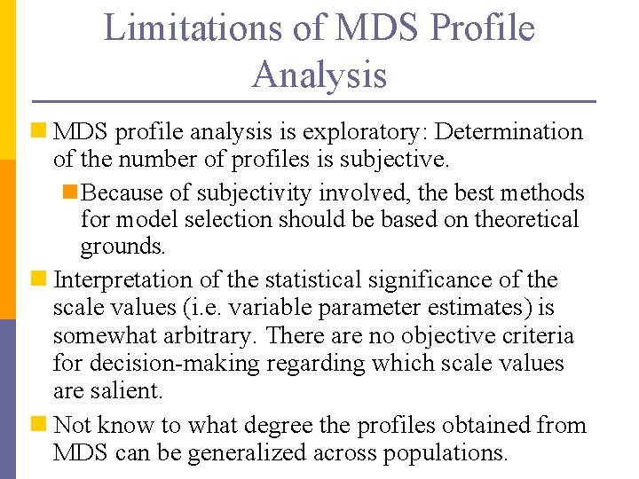
Limitations of MDS Profile Analysis n MDS profile analysis is exploratory: Determination of the number of profiles is subjective. n Because of subjectivity involved, the best methods for model selection should be based on theoretical grounds. n Interpretation of the statistical significance of the scale values (i. e. variable parameter estimates) is somewhat arbitrary. There are no objective criteria for decision-making regarding which scale values are salient. n Not know to what degree the profiles obtained from MDS can be generalized across populations.