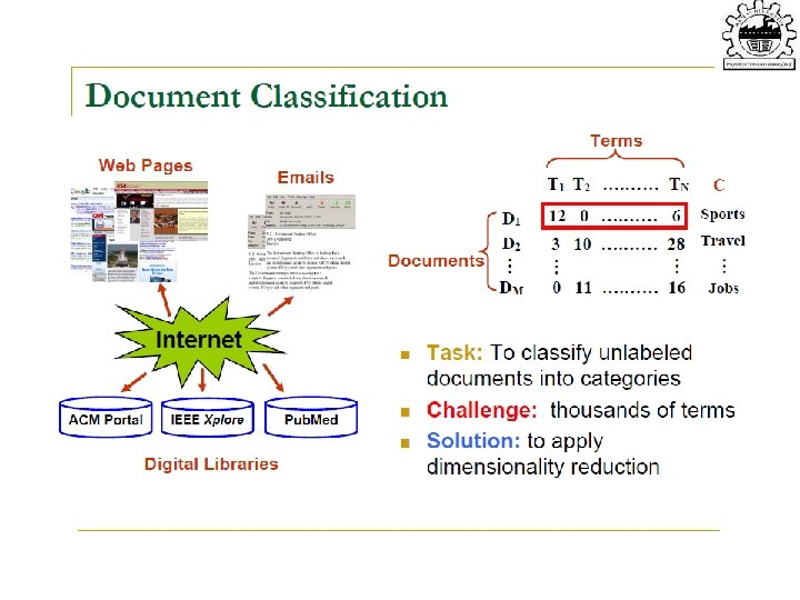
Curse of Dimensionality Dimensionality Reduction Why Reduce Dimensionality


 variables • Goal: Characterize dependency among")
 variables generating d observables •")


 are chosen")


 • Multiple sensors receiving signals which")
 Assumption: The observed data is the sum of a set")


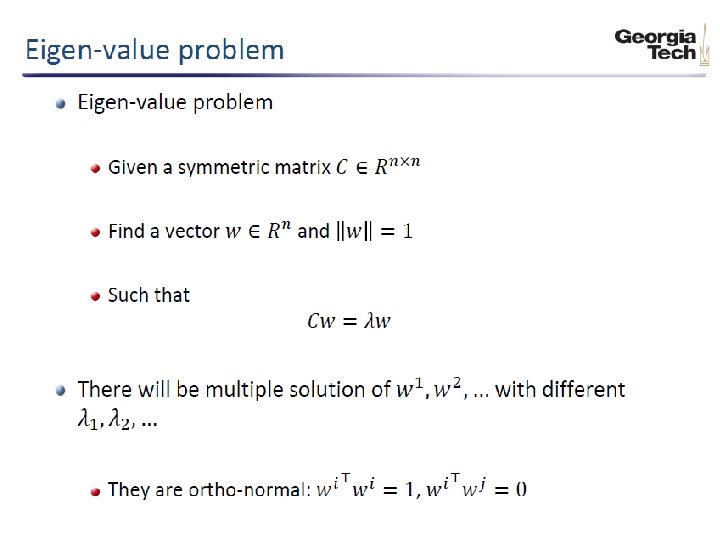
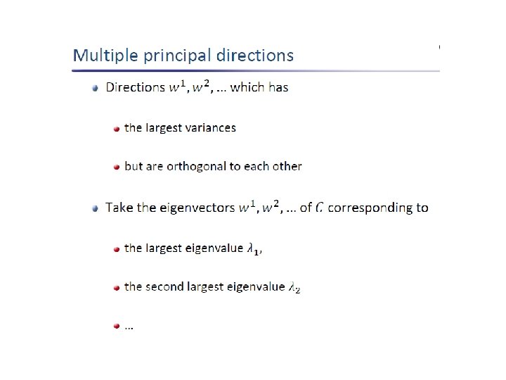
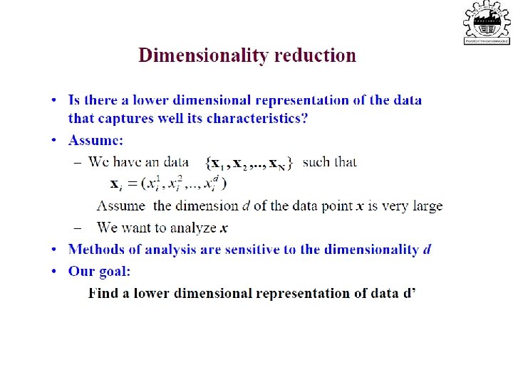
 • Find a low-dimensional space such that when x is")
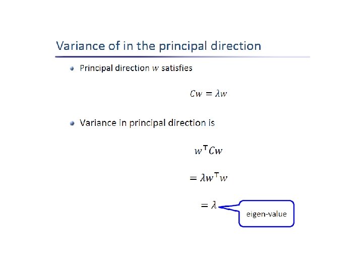
 subject to ||w||=1 ∑w 1 = αw 1 that is,")
 where the columns of W are")
 explained when λi")

- Slides: 98
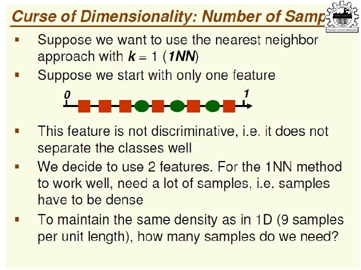
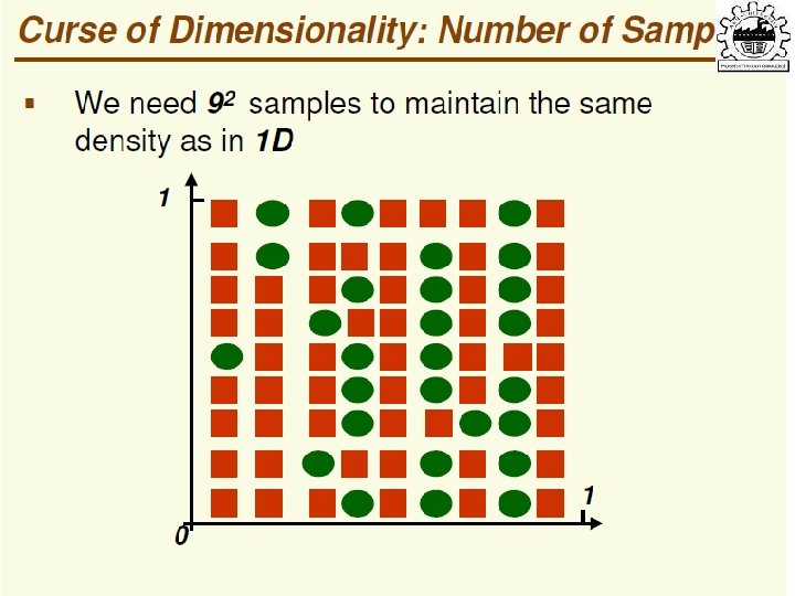
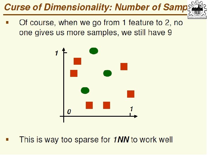
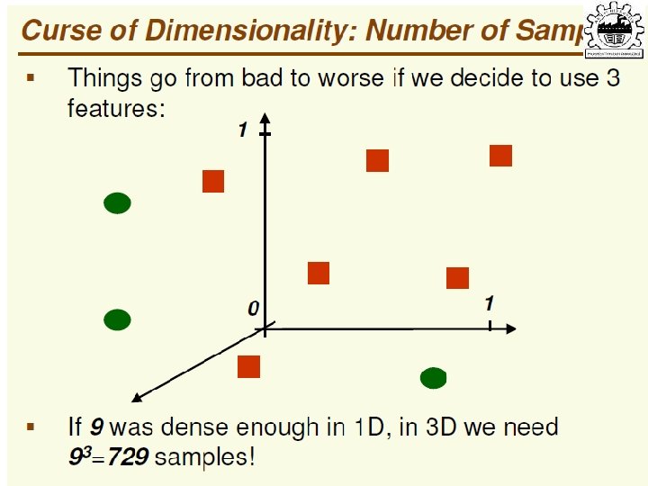
Curse of Dimensionality
Dimensionality Reduction
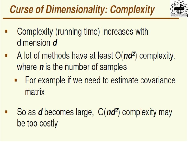
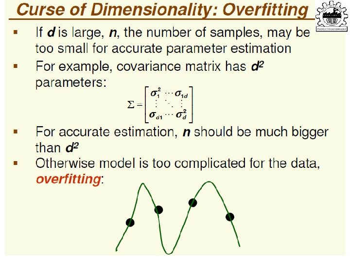
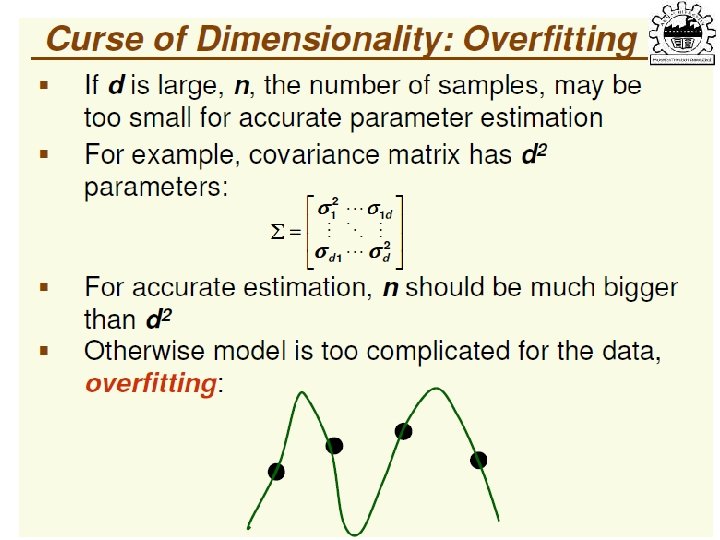
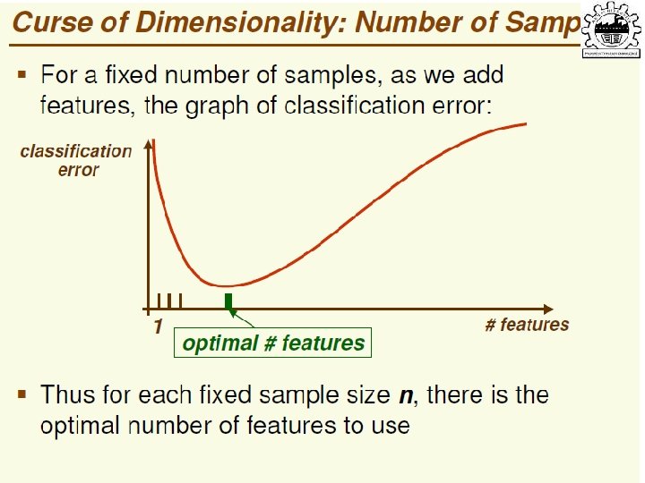
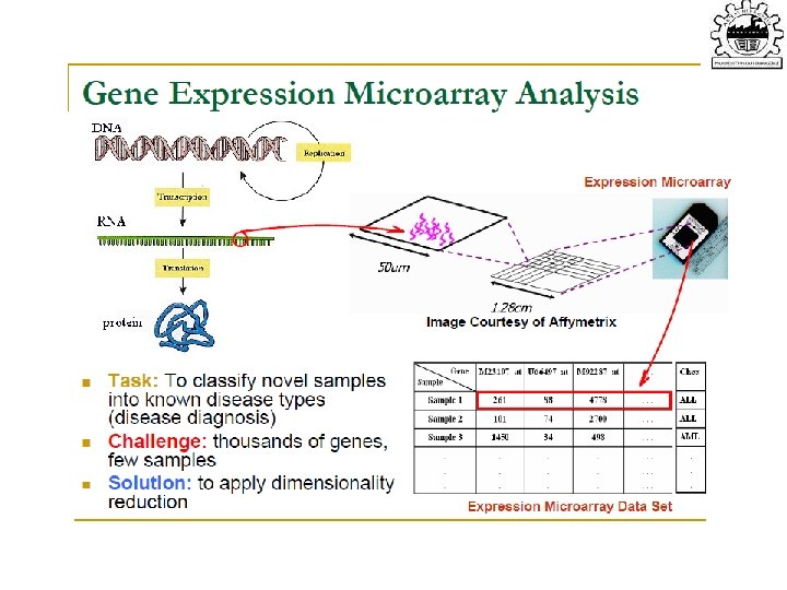
Why Reduce Dimensionality? Reduces time complexity: Less computation Reduces space complexity: Less parameters Saves the cost of observing the feature Simpler models are more robust on small datasets • More interpretable; simpler explanation • Data visualization (structure, groups, outliers, etc) if plotted in 2 or 3 dimensions • • Lecture Notes for E Alpaydın 2010 Introduction to Machine Learning 2 e © The MIT Press (V 1. 0) 24
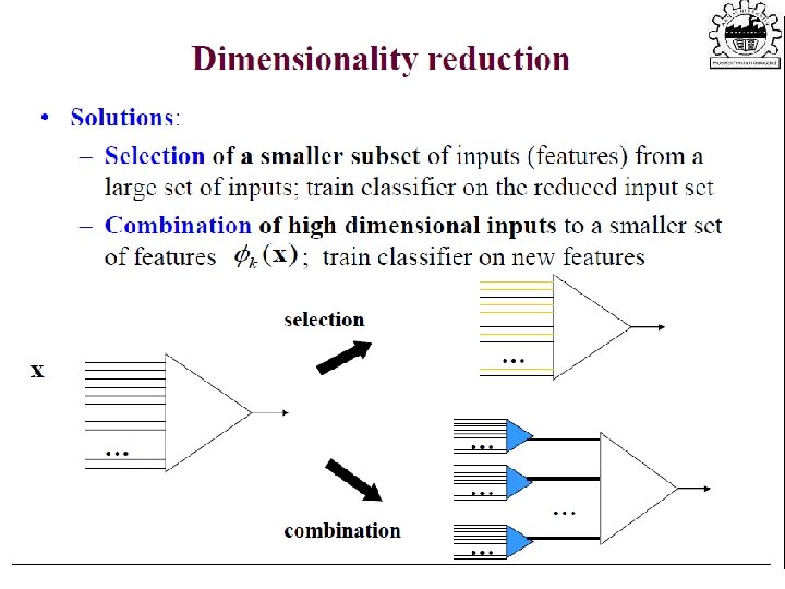
Feature Selection vs Extraction • Feature selection: Choosing k<d important features, ignoring the remaining d – k Subset selection algorithms • Feature extraction: Project the original xi , i =1, . . . , d dimensions to new k<d dimensions, zj , j =1, . . . , k Principal components analysis (PCA), linear discriminant analysis (LDA), factor analysis (FA) Lecture Notes for E Alpaydın 2010 Introduction to Machine Learning 2 e © The MIT Press (V 1. 0) 31
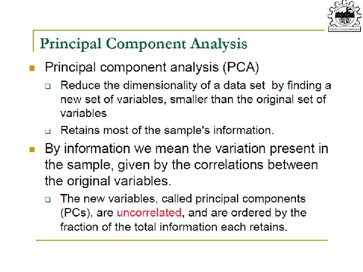
Principal Component Analysis
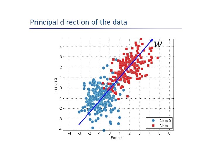
PCA • Intuition: find the axis that shows the greatest variation, and project all points into this axis f 2 e 1 e 2 f 1
Factor Analysis
Introduction • The purpose of factor analysis is to describe the variation among many variables in terms of a few underlying but unobservable random variables called factors • All the covariance or correlations are explained by the common factors • Any portion of the variance unexplained by the common factors is assigned to residual errors terms which are called unique factors
Factor Analysis • Factor analysis is a class of procedures used for data reduction and summarization. • It is an interdependence technique: no distinction between dependent and independent variables. • Factor analysis is used: – To identify underlying dimensions, or factors, that explain the correlations among a set of variables. – To identify a new, smaller, set of uncorrelated variables to replace the original set of correlated variables.
Concept • Factor analysis can be viewed as a statistical procedure for grouping variables into subsets such that the variables with each set are mutually highly correlated, whereas at the same time variables in different subsets are relatively uncorrelated.
Factor Analysis • Assume set of unobservable (“latent”) variables • Goal: Characterize dependency among observables using latent variables • Suppose group of variables having large correlation among themselves and small correlation with other variables • Single factor? 51
Factor Analysis • Assume k input factors (latent unobservable) variables generating d observables • Assume all variations in observable variables are due to latent or noise (with unknown variance) • Find transformation from unobservable to observables which explain the data 52
What is FA? • Patterns of correlations are identified and either used as descriptives (PCA) or as indicative of underlying theory (FA) • Process of providing an operational definition for latent construct (through regression equation)
Factor Analysis Model Each variable is expressed as a linear combination of factors. The factors are some common factors plus a unique factor. The factor model is represented as: Xi = Ai 1 F 1 + Ai 2 F 2 + Ai 3 F 3 +. . . + Aim. Fm + Vi. Ui where Xi Aij Fj Vi U i m = i th standardized variable = standardized mult reg coeff of var i on common factor j = standardized reg coeff of var i on unique factor i = the unique factor for variable i = number of common factors
Factor Analysis Model • The first set of weights (factor score coefficients) are chosen so that the first factor explains the largest portion of the total variance. • Then a second set of weights can be selected, so that the second factor explains most of the residual variance, subject to being uncorrelated with the first factor. • This same principle applies for selecting additional weights for the additional factors.
Factor Analysis Model The common factors themselves can be expressed as linear combinations of the observed variables. Fi = Wi 1 X 1 + Wi 2 X 2 + Wi 3 X 3 +. . . + Wik. Xk Where: Fi = estimate of i th factor Wi= weight or factor score coefficient k = number of variables
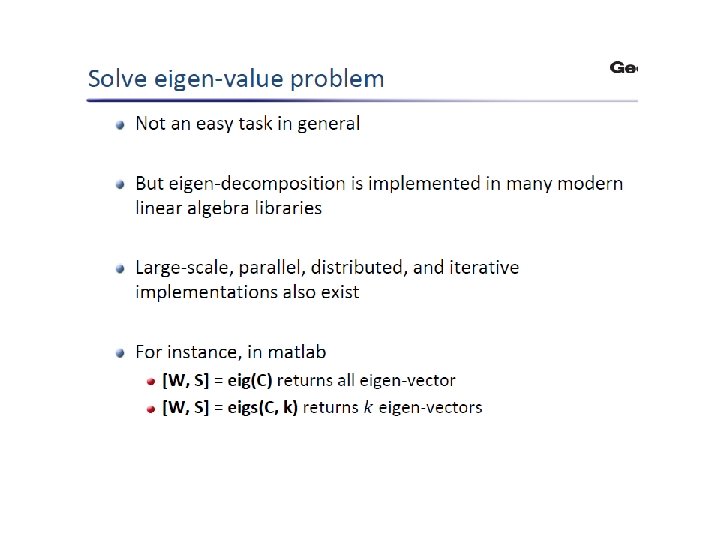
Factor Analysis • Find V such that where S is estimation of covariance matrix and V loading (explanation by latent variables) • V is d x k matrix (k<d) • Solution using eigenvalue and eigenvectors 57
Conducting Factor Analysis Fig. 19. 2 Problem formulation Construction of the Correlation Matrix Method of Factor Analysis Determination of Number of Factors Rotation of Factors Interpretation of Factors Calculation of Factor Scores Determination of Model Fit
General Steps to FA • Step 1: Selecting and Measuring a set of variables in a given domain • Step 2: Data screening in order to prepare the correlation matrix • Step 3: Factor Extraction • Step 4: Factor Rotation to increase interpretability • Step 5: Interpretation • Further Steps: Validation and Reliability of the measures
Factor Analysis • In FA, factors zj are stretched, rotated and translated to generate x 60
FA Usage Speech is a function of position of small number of articulators (lungs, lips, tongue) Factor analysis: go from signal space (4000 points for 500 ms ) to articulation space (20 points) Classify speech (assign text label) by 20 points Speech Compression: send 20 values 61
Independent Component Analysis
Motivation • Method for finding underlying components from multi-dimensional data • Focus is on Independent and Non-Gaussian components in ICA as compared to uncorrelated and gaussian components in FA and PCA Sep 10, 2003 ENEE 698 A Seminar 63
Cocktail-party Problem • Multiple speakers in room (independent) • Multiple sensors receiving signals which are mixture of original signals • Estimate original source signals from mixture of received signals • Can be viewed as Blind-Source Separation as mixing parameters are not known Sep 10, 2003 ENEE 698 A Seminar 64
Independent Components Analysis (ICA) Assumption: The observed data is the sum of a set of inputs which have been mixed together in an unknown fashion. The goal of ICA is to discover both the inputs and how they were mixed. FMRI – Week 10 – Analysis II Mc. Keown, et al. (1998)
PCA finds the directions of maximum variance ICA finds the directions of maximum independence
Principle: Maximize Information • Q: How to extract maximum information from multiple visual channels? • A: ICA does this -- it maximizes joint entropy & minimizes mutual information between output channels (Bell & Sejnowski, 1995). • ICA produces brain-like visual filters for natural images. Set of 144 ICA filters
Principles of ICA Estimation • “Nongaussian is independent”: central limit theorem • Measure of nonguassianity – Kurtosis: (Kurtosis=0 for a gaussian distribution) – Negentropy: a gaussian variable has the largest entropy among all random variables of equal variance:
ICA Definition • Observe n random variables which are linear combinations of n random variables which are mutually independent • • In Matrix Notation, X = AS Assume source signals are statistically independent Estimate the mixing parameters and source signals Find a linear transformation of observed signals such that the resulting signals are as independent as possible Sep 10, 2003 ENEE 698 A Seminar 69
Restrictions and Ambiguities • Components are assumed independent • Components must have non-gaussian densities • Energies of independent components can’t be estimated • Sign Ambiguity in independent components Sep 10, 2003 ENEE 698 A Seminar 70
Gaussian and Non-Gaussian components • If some components are gaussian and some are non-gaussian. – Can estimate all non-gaussian components – Linear combination of gaussian components can be estimated. – If only one gaussian component, model can be estimated Sep 10, 2003 ENEE 698 A Seminar 71
Why Non-Gaussian Components • Uncorrelated Gaussian r. v. are independent • Orthogonal mixing matrix can’t be estimated from Gaussian r. v. • For Gaussian r. v. estimate of model is up to an orthogonal transformation • ICA can be considered as non-gaussian factor analysis Sep 10, 2003 ENEE 698 A Seminar 72
Summing up
The Factor Analysis Model • The generative model for factor analysis assumes that the data was produced in three stages: – Pick values independently for some hidden factors that have Gaussian priors j – Linearly combine the factors using a factor loading matrix. Use more linear combinations than factors. – Add Gaussian noise that is different for each input. i
The Full Gaussian Model • The generative model for factor analysis assumes that the data was produced in three stages: – Pick values independently for some hidden factors that have Gaussian priors – Linearly combine the factors using a square matrix. – There is no need to add Gaussian noise because we can already generate all points in the dataspace. j i
The PCA Model • The generative model for factor analysis assumes that the data was produced in three stages: – Pick values independently for some hidden factors that can have any value j – Linearly combine the factors using a factor loading matrix. Use more linear combinations than factors. – Add Gaussian noise that is the same for each input. i
The Probabilistic PCA Model • The generative model for factor analysis assumes that the data was produced in three stages: – Pick values independently for some hidden factors that can have any value j – Linearly combine the factors using a factor loading matrix. Use more linear combinations than factors. – Add Gaussian noise that is the same for each input. i
Extra slides
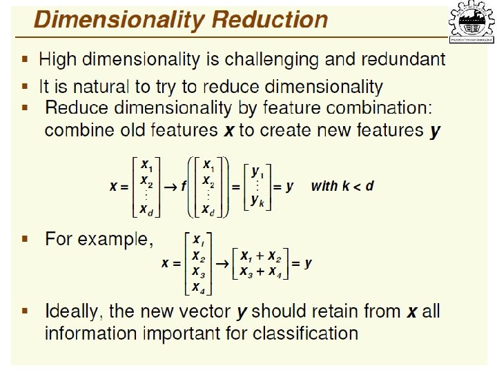
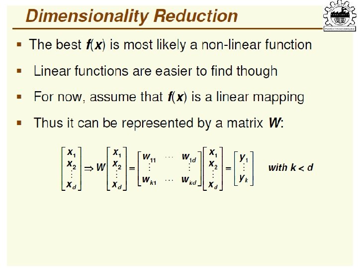
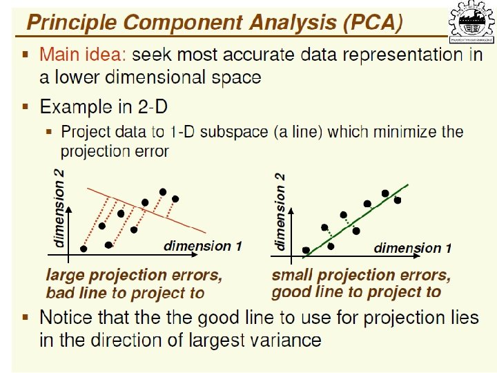
Dimensionality Reduction • One approach to deal with high dimensional data is by reducing their dimensionality. • Project high dimensional data onto a lower dimensional sub -space using linear or non-linear transformations.
Dimensionality Reduction • Linear transformations are simple to compute and tractable. kx 1 kxd dx 1 (k<<d) • Classical –linear- approaches: – Principal Component Analysis (PCA) – Fisher Discriminant Analysis (FDA) –Singular Value Decomosition (SVD) --Factor Analysis (FA) --Canonical Correlation(CCA)
Principal Component Analysis 81
Principal Component Analysis This function is minimized if xo is equal to mean 82
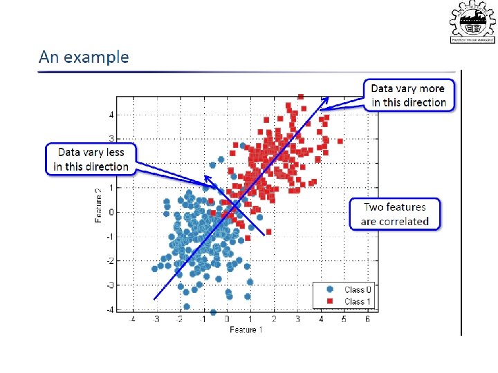
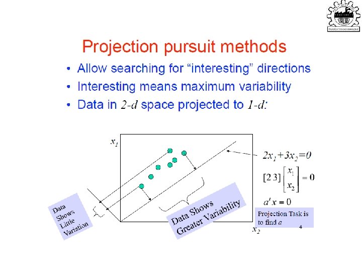
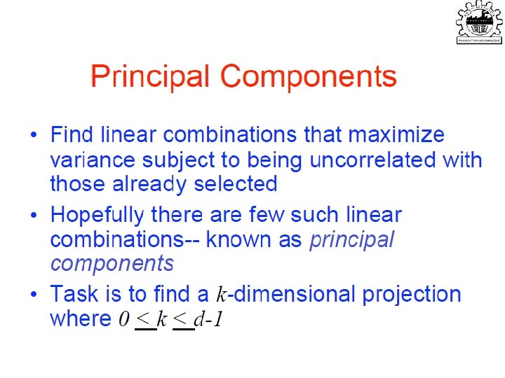
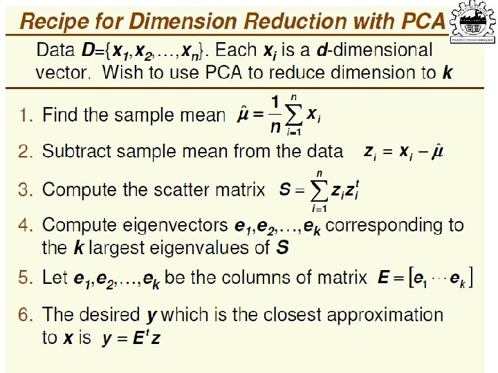
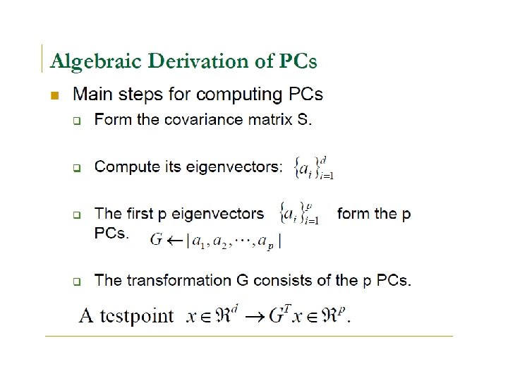
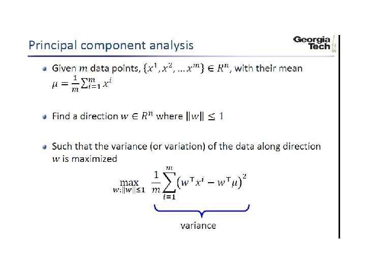
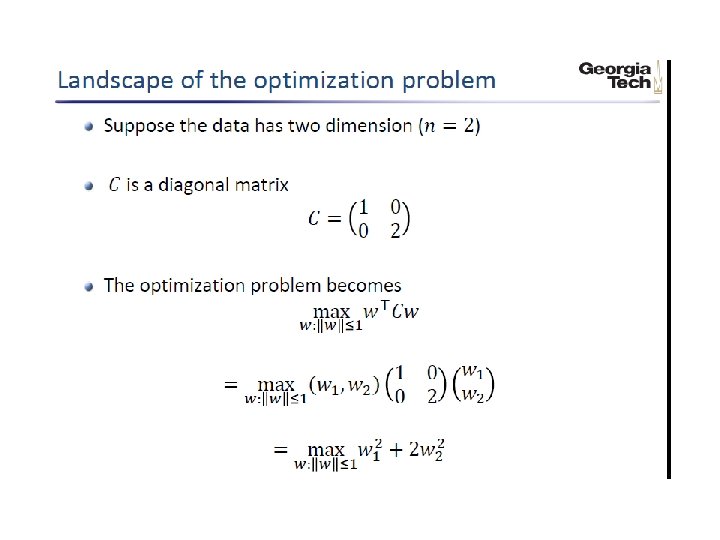
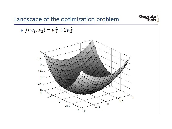
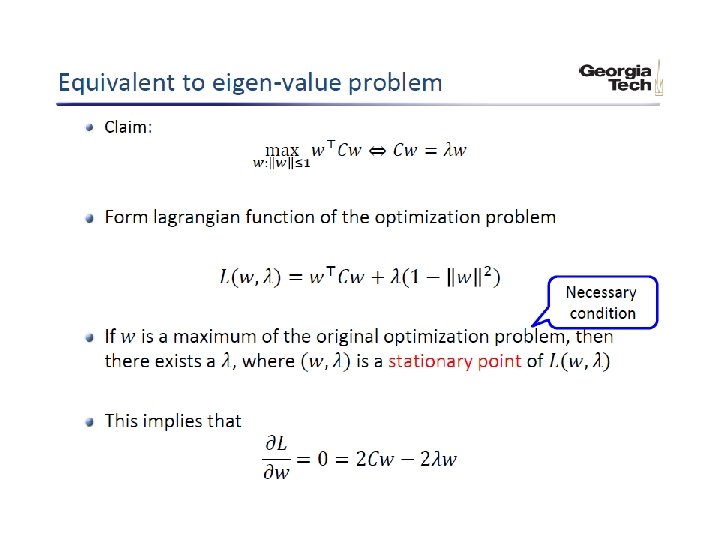
Principal Components Analysis (PCA) • Find a low-dimensional space such that when x is projected there, information loss is minimized. • The projection of x on the direction of w is: z = w. T x • Find w such that Var(z) is maximized Var(z) = Var(w. Tx) = E[(w. Tx – w. Tμ)2] = E[(w. Tx – w. Tμ)] = E[w. T(x – μ)Tw] = w. T E[(x – μ)(x –μ)T]w = w. T ∑ w where Var(x)= E[(x – μ)(x –μ)T] = ∑ Lecture Notes for E Alpaydın 2010 Introduction to Machine Learning 2 e © The MIT Press (V 1. 0) 94
• Maximize Var(z) subject to ||w||=1 ∑w 1 = αw 1 that is, w 1 is an eigenvector of ∑ Choose the one with the largest eigenvalue for Var(z) to be max • Second principal component: Max Var(z 2), s. t. , ||w 2||=1 and orthogonal to w 1 ∑ w 2 = α w 2 that is, w 2 is another eigenvector of ∑ and so on. Lecture Notes for E Alpaydın 2010 Introduction to Machine Learning 2 e © The MIT Press (V 1. 0) 95
What PCA does z = WT(x – m) where the columns of W are the eigenvectors of ∑, and m is sample mean Centers the data at the origin and rotates the axes Lecture Notes for E Alpaydın 2010 Introduction to Machine Learning 2 e © The MIT Press (V 1. 0) 96
How to choose k ? • Proportion of Variance (Po. V) explained when λi are sorted in descending order • Typically, stop at Po. V>0. 9 • Scree graph plots of Po. V vs k, stop at “elbow” Lecture Notes for E Alpaydın 2010 Introduction to Machine Learning 2 e © The MIT Press (V 1. 0) 97
Factor Analysis • In FA, factors zj are stretched, rotated and translated to generate x Lecture Notes for E Alpaydın 2010 Introduction to Machine Learning 2 e © The MIT Press (V 1. 0) 98