Multimedia Indexing and Dimensionality Reduction Multimedia Data Management

Multimedia Indexing and Dimensionality Reduction

Multimedia Data Management • The need to query and analyze vast amounts of multimedia data (i. e. , images, sound tracks, video tracks) has increased in the recent years. • Joint Research from Database Management, Computer Vision, Signal Processing and Pattern Recognition aims to solve problems related to multimedia data management.

Multimedia Data • There are four major types of multimedia data: images, video sequences, sound tracks, and text. • From the above, the easiest type to manage is text, since we can order, index, and search text using string management techniques, etc. • Management of simple sounds is also possible by representing audio as signal sequences over different channels. • Image retrieval has received a lot of attention in the last decade (CV and DBs). The main techniques can be extended and applied also for video retrieval.

Content-based Image Retrieval • Images were traditionally managed by first annotating their contents and then using text-retrieval techniques to index them. • However, with the increase of information in digital image format some drawbacks of this technique were revealed: • Manual annotation requires vast amount of labor • Different people may perceive differently the contents of an image; thus no objective keywords for search are defined • A new research field was born in the 90’s: Contentbased Image Retrieval aims at indexing and retrieving images based on their visual contents.

Feature Extraction • The basis of Content-based Image Retrieval is to extract and index some visual features of the images. • There are general features (e. g. , color, texture, shape, etc. ) and domain-specific features (e. g. , objects contained in the image). • Domain-specific feature extraction can vary with the application domain and is based on pattern recognition • On the other hand, general features can be used independently from the image domain.

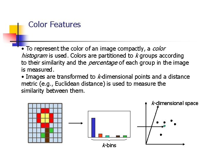
Color Features • To represent the color of an image compactly, a color histogram is used. Colors are partitioned to k groups according to their similarity and the percentage of each group in the image is measured. • Images are transformed to k-dimensional points and a distance metric (e. g. , Euclidean distance) is used to measure the similarity between them. k-dimensional space k-bins

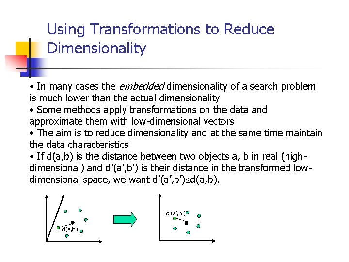
Using Transformations to Reduce Dimensionality • In many cases the embedded dimensionality of a search problem is much lower than the actual dimensionality • Some methods apply transformations on the data and approximate them with low-dimensional vectors • The aim is to reduce dimensionality and at the same time maintain the data characteristics • If d(a, b) is the distance between two objects a, b in real (highdimensional) and d’(a’, b’) is their distance in the transformed lowdimensional space, we want d’(a’, b’) d(a, b)

Problem - Motivation n n Given a database of documents, find documents containing “data”, “retrieval” Applications: n Web n law + patent offices n digital libraries n information filtering

Problem - Motivation n n Types of queries: n boolean (‘data’ AND ‘retrieval’ AND NOT. . . ) n additional features (‘data’ ADJACENT ‘retrieval’) n keyword queries (‘data’, ‘retrieval’) How to search a large collection of documents?

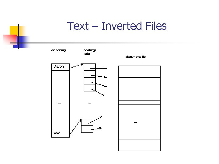
Text – Inverted Files

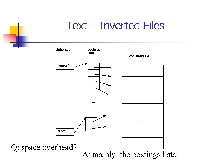
Text – Inverted Files Q: space overhead? A: mainly, the postings lists

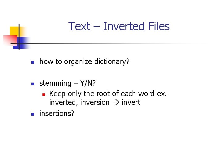
Text – Inverted Files n n n how to organize dictionary? stemming – Y/N? n Keep only the root of each word ex. inverted, inversion invert insertions?

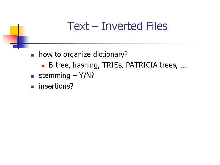
Text – Inverted Files n n n how to organize dictionary? n B-tree, hashing, TRIEs, PATRICIA trees, . . . stemming – Y/N? insertions?

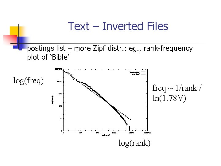
Text – Inverted Files n postings list – more Zipf distr. : eg. , rank-frequency plot of ‘Bible’ log(freq) freq ~ 1/rank / ln(1. 78 V) log(rank)

Text – Inverted Files n postings lists n Cutting+Pedersen n (keep first 4 in B-tree leaves) n how to allocate space: [Faloutsos+92] n geometric progression n compression (Elias codes) [Zobel+] – down to 2% overhead! n Conclusions: needs space overhead (2%-300%), but it is the fastest

Text - Detailed outline n Text databases n n n problem full text scanning inversion signature files (a. k. a. Bloom Filters) Vector model and clustering information filtering and LSI

Vector Space Model and Clustering n n Keyword (free-text) queries (vs Boolean) each document: -> vector (HOW? ) each query: -> vector search for ‘similar’ vectors

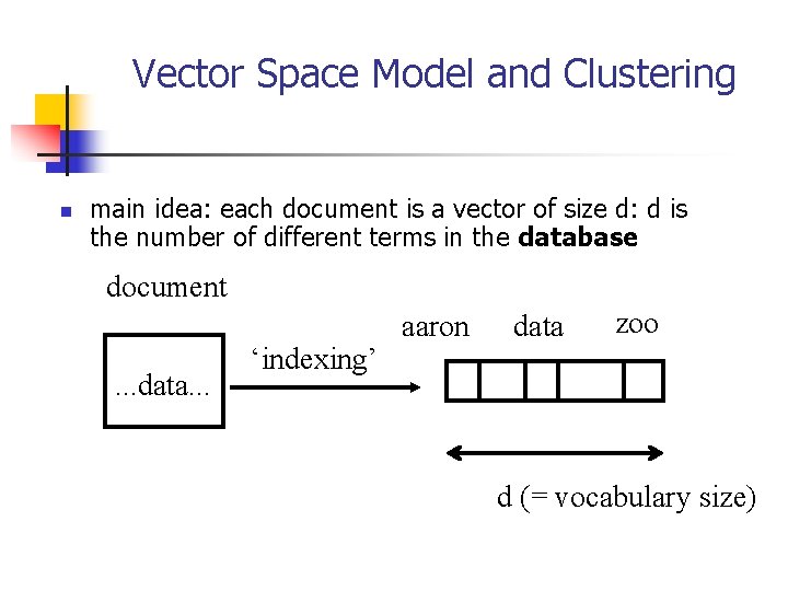
Vector Space Model and Clustering n main idea: each document is a vector of size d: d is the number of different terms in the database document. . . data. . . ‘indexing’ aaron data zoo d (= vocabulary size)

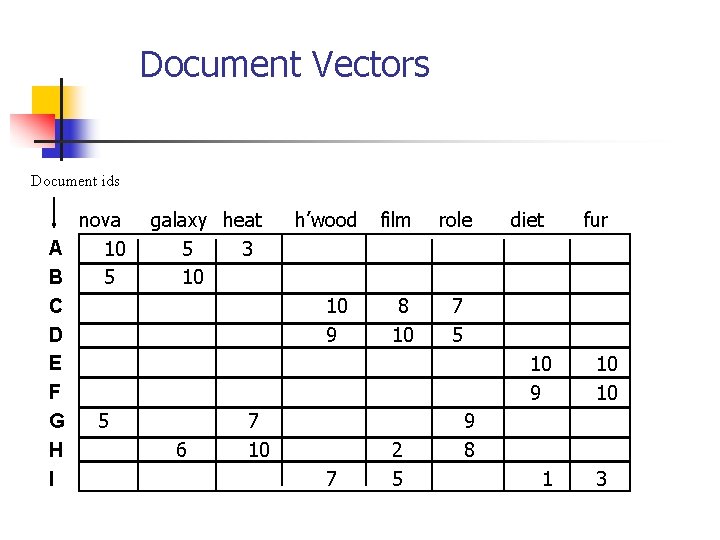
Document Vectors Documents are represented as “bags of words” OR as vectors. n n n A vector is like an array of floating points Has direction and magnitude Each vector holds a place for every term in the collection Therefore, most vectors are sparse

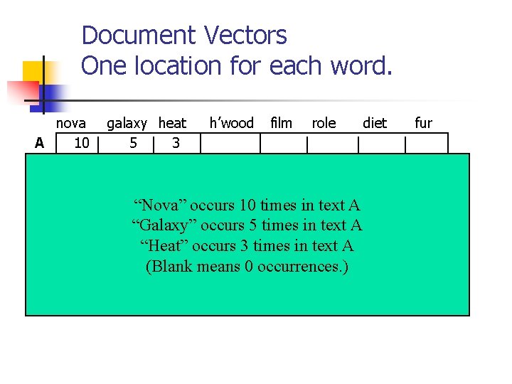
Document Vectors One location for each word. nova A 10 B 5 C D E F G 5 H I galaxy heat 5 3 10 h’wood film 10 occurs 910 8 10 times role diet 7 5 text “Nova” in A “Galaxy” occurs 5 times in text A 10 “Heat” occurs 3 times in text A 9 7 means 0 occurrences. ) 9 (Blank 6 10 7 2 5 fur 10 10 8 1 3

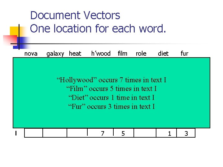
Document Vectors One location for each word. nova A 10 B 5 C D E F G 5 H I galaxy heat 5 3 10 h’wood film role diet “Hollywood” occurs 78 times 7 in text I 10 “Film” occurs 9 5 times 10 in 5 text I “Diet” occurs 1 time in text I 10 “Fur” occurs 3 times in text I 9 6 7 10 7 2 5 fur 10 10 9 8 1 3

Document Vectors Document ids nova A 10 B 5 C D E F G 5 H I galaxy heat 5 3 10 h’wood 10 9 film 8 10 role diet 7 5 10 9 6 7 10 7 2 5 fur 10 10 9 8 1 3

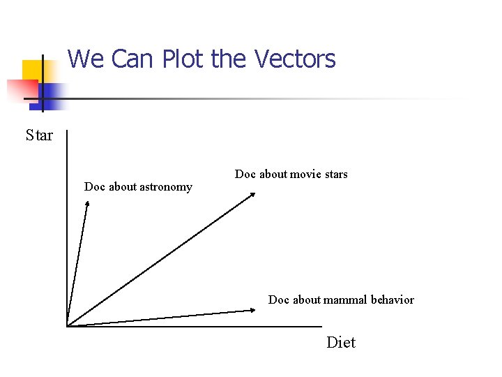
We Can Plot the Vectors Star Doc about astronomy Doc about movie stars Doc about mammal behavior Diet

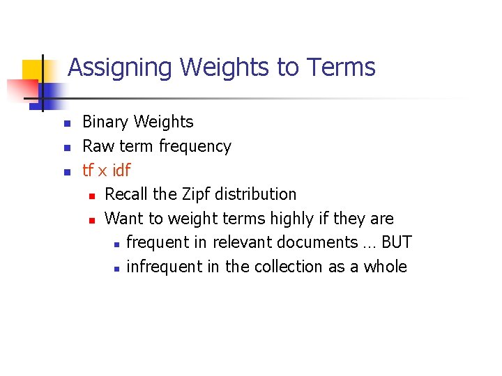
Assigning Weights to Terms n n n Binary Weights Raw term frequency tf x idf n Recall the Zipf distribution n Want to weight terms highly if they are n frequent in relevant documents … BUT n infrequent in the collection as a whole

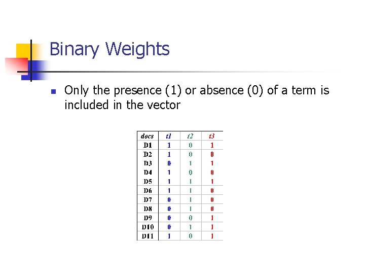
Binary Weights n Only the presence (1) or absence (0) of a term is included in the vector

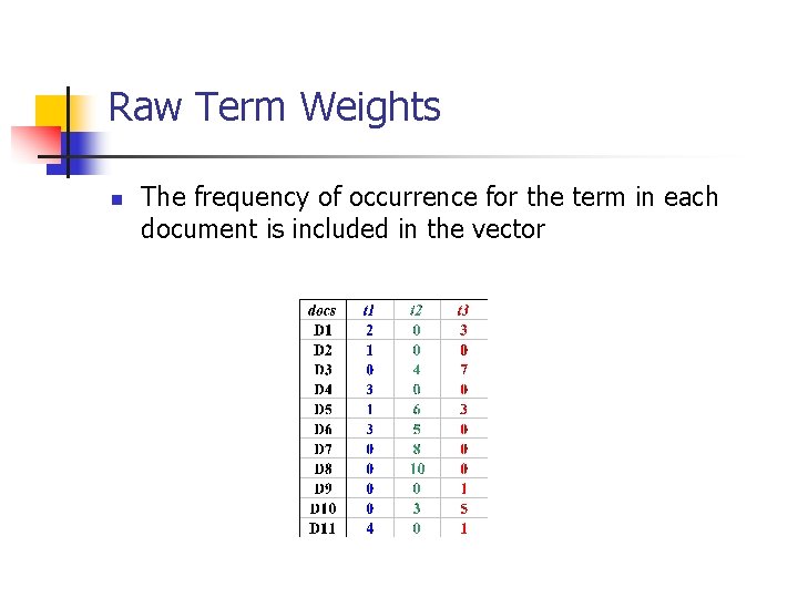
Raw Term Weights n The frequency of occurrence for the term in each document is included in the vector

Assigning Weights n n tf x idf measure: n term frequency (tf) n inverse document frequency (idf) -- a way to deal with the problems of the Zipf distribution Goal: assign a tf * idf weight to each term in each document

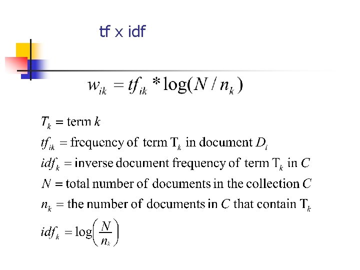
tf x idf

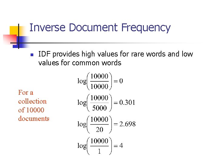
Inverse Document Frequency n IDF provides high values for rare words and low values for common words For a collection of 10000 documents

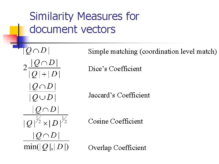
Similarity Measures for document vectors Simple matching (coordination level match) Dice’s Coefficient Jaccard’s Coefficient Cosine Coefficient Overlap Coefficient

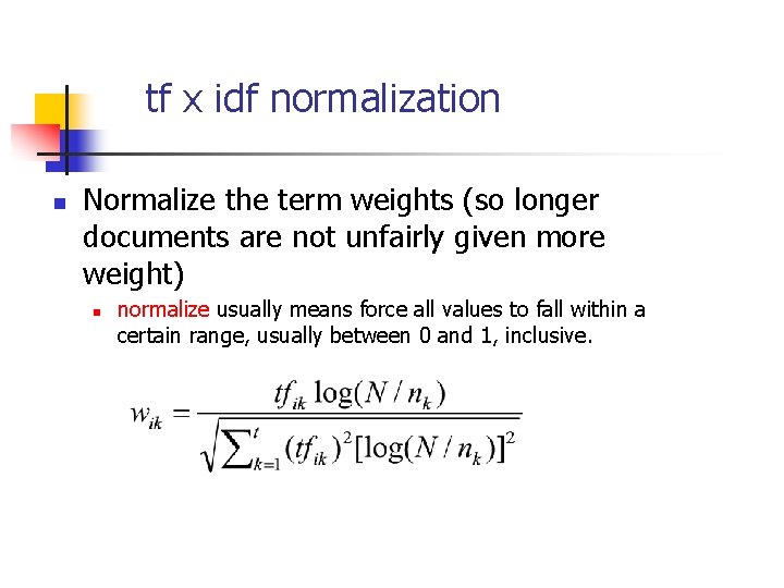
tf x idf normalization n Normalize the term weights (so longer documents are not unfairly given more weight) n normalize usually means force all values to fall within a certain range, usually between 0 and 1, inclusive.

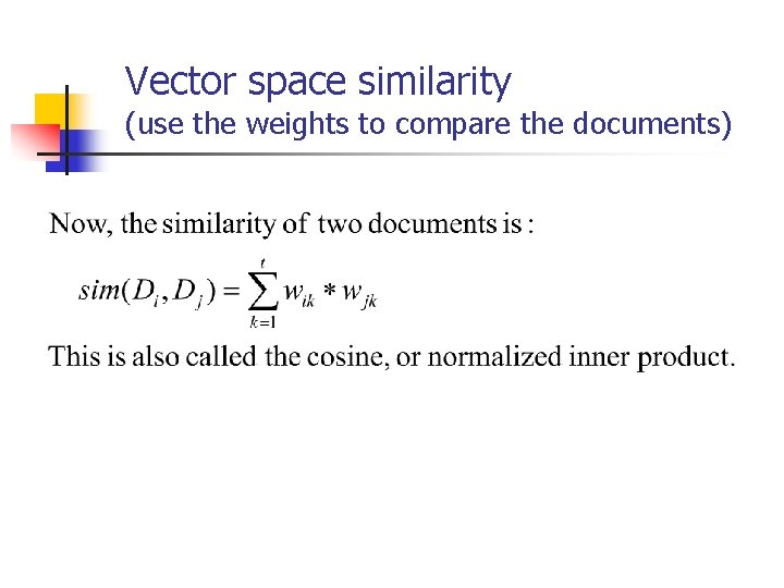
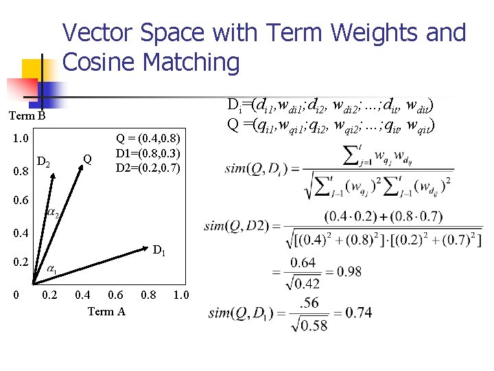
Vector space similarity (use the weights to compare the documents)

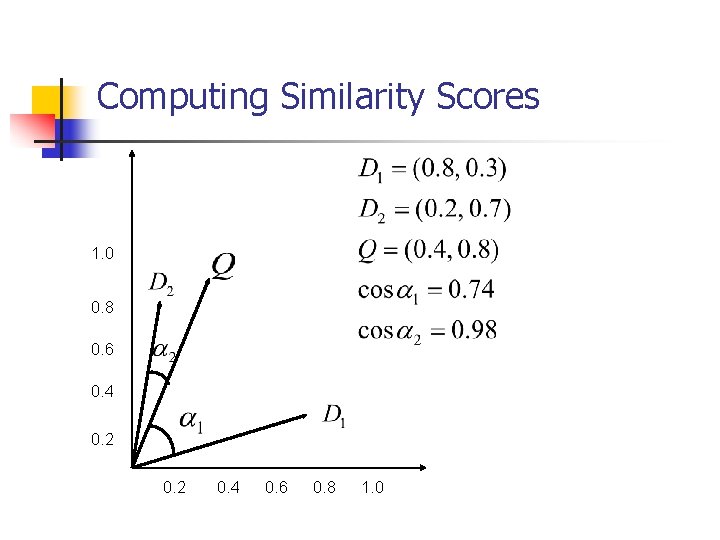
Computing Similarity Scores 1. 0 0. 8 0. 6 0. 4 0. 2 0. 4 0. 6 0. 8 1. 0

Vector Space with Term Weights and Cosine Matching Term B 1. 0 0. 8 D 2 Q Q = (0. 4, 0. 8) D 1=(0. 8, 0. 3) D 2=(0. 2, 0. 7) 0. 6 0. 4 D 1 0. 2 0. 4 0. 6 Term A 0. 8 1. 0 Di=(di 1, wdi 1; di 2, wdi 2; …; dit, wdit) Q =(qi 1, wqi 1; qi 2, wqi 2; …; qit, wqit)

Text - Detailed outline n Text databases n n n problem full text scanning inversion signature files (a. k. a. Bloom Filters) Vector model and clustering information filtering and LSI

Information Filtering + LSI n [Foltz+, ’ 92] Goal: n n n users specify interests (= keywords) system alerts them, on suitable newsdocuments Major contribution: LSI = Latent Semantic Indexing n latent (‘hidden’) concepts

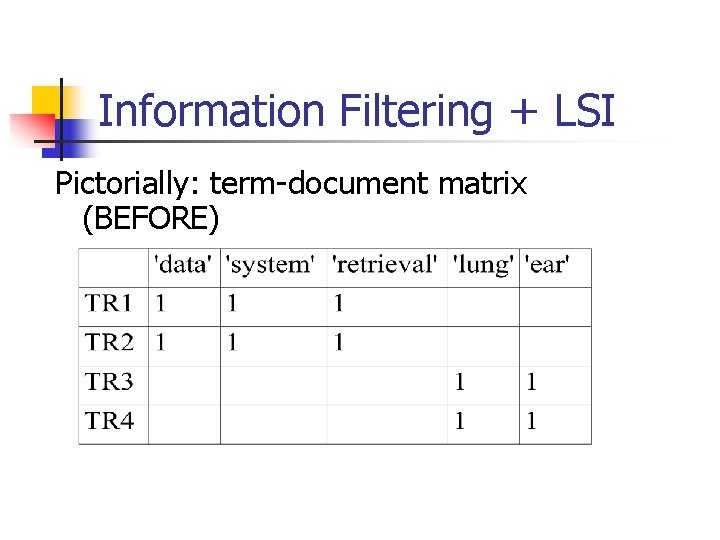
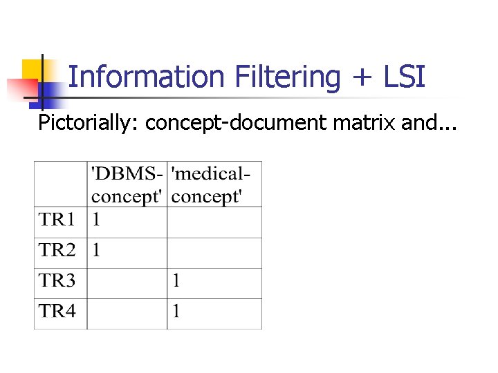
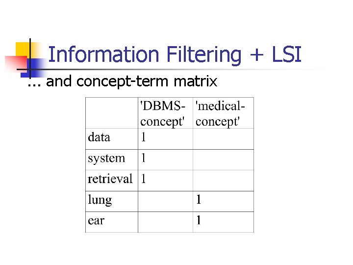
Information Filtering + LSI Main idea n map each document into some ‘concepts’ n map each term into some ‘concepts’ ‘Concept’: ~ a set of terms, with weights, e. g. n “data” (0. 8), “system” (0. 5), “retrieval” (0. 6) -> DBMS_concept

Information Filtering + LSI Pictorially: term-document matrix (BEFORE)

Information Filtering + LSI Pictorially: concept-document matrix and. . .

Information Filtering + LSI. . . and concept-term matrix

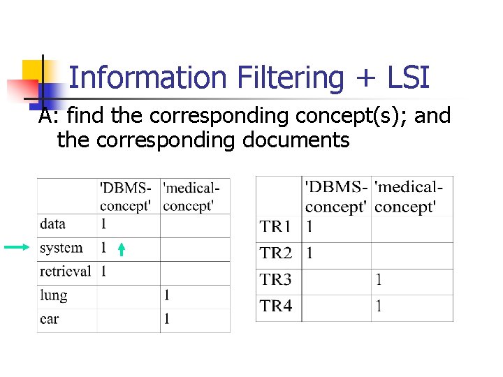
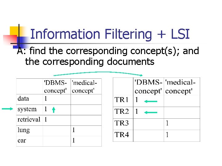
Information Filtering + LSI Q: How to search, eg. , for ‘system’?

Information Filtering + LSI A: find the corresponding concept(s); and the corresponding documents

Information Filtering + LSI A: find the corresponding concept(s); and the corresponding documents

Information Filtering + LSI Thus it works like an (automatically constructed) thesaurus: we may retrieve documents that DON’T have the term ‘system’, but they contain almost everything else (‘data’, ‘retrieval’)

SVD - Detailed outline n n n Motivation Definition - properties Interpretation Complexity Case studies Additional properties

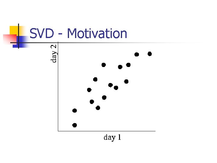
SVD - Motivation n n problem #1: text - LSI: find ‘concepts’ problem #2: compression / dim. reduction

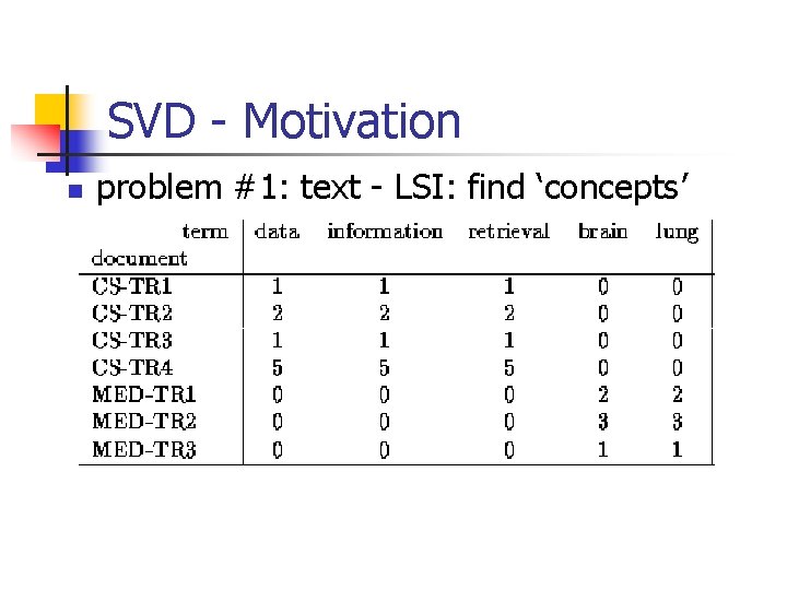
SVD - Motivation n problem #1: text - LSI: find ‘concepts’

SVD - Motivation n problem #2: compress / reduce dimensionality

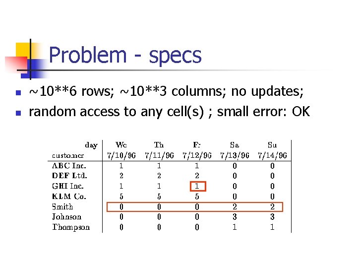
Problem - specs n n ~10**6 rows; ~10**3 columns; no updates; random access to any cell(s) ; small error: OK

SVD - Motivation

SVD - Motivation

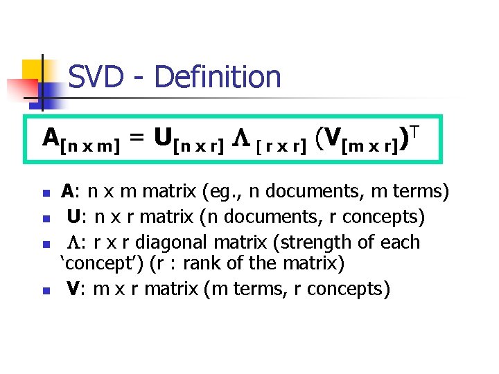
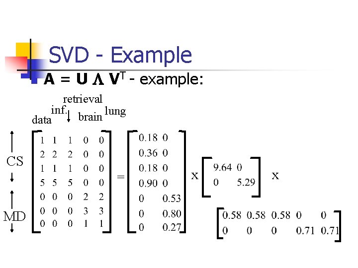
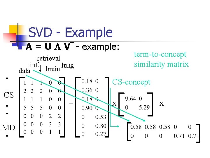
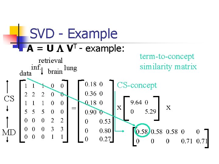
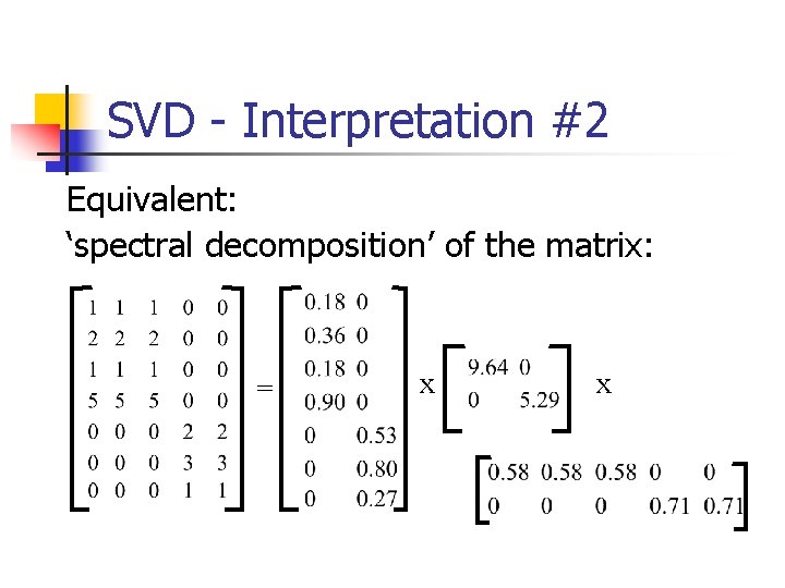
SVD - Definition A[n x m] = U[n x r] L [ r x r] (V[m x r])T n n A: n x m matrix (eg. , n documents, m terms) U: n x r matrix (n documents, r concepts) L: r x r diagonal matrix (strength of each ‘concept’) (r : rank of the matrix) V: m x r matrix (m terms, r concepts)

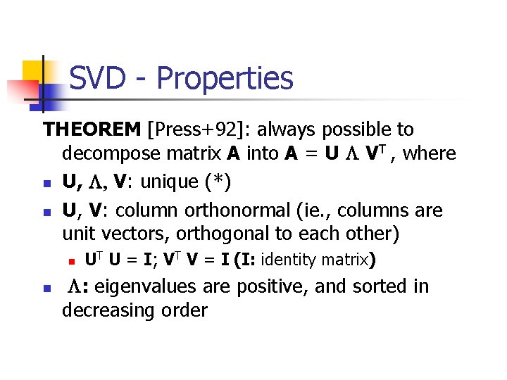
SVD - Properties THEOREM [Press+92]: always possible to decompose matrix A into A = U L VT , where n U, L, V: unique (*) n U, V: column orthonormal (ie. , columns are unit vectors, orthogonal to each other) n n UT U = I; VT V = I (I: identity matrix) L: eigenvalues are positive, and sorted in decreasing order

SVD - Example n A = U L VT - example: retrieval inf. lung brain data CS = MD x x

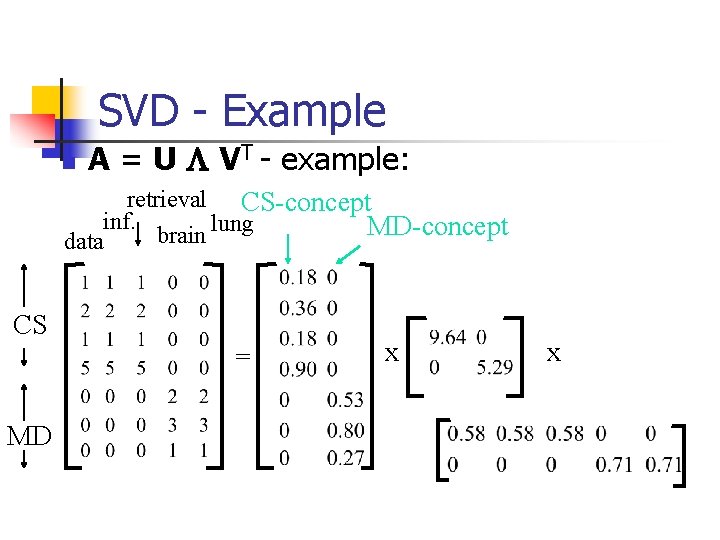
SVD - Example n A = U L VT - example: retrieval CS-concept inf. lung MD-concept brain data CS = MD x x

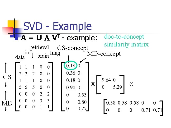
SVD - Example n A = U L VT - example: doc-to-concept similarity matrix retrieval CS-concept inf. lung MD-concept brain data CS = MD x x

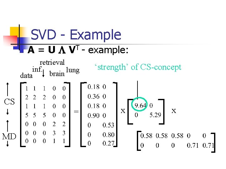
SVD - Example n A = U L VT - example: retrieval inf. lung brain data CS = MD ‘strength’ of CS-concept x x

SVD - Example n A = U L VT - example: retrieval inf. lung brain data term-to-concept similarity matrix CS-concept CS = MD x x

SVD - Example n A = U L VT - example: retrieval inf. lung brain data term-to-concept similarity matrix CS-concept CS = MD x x

SVD - Detailed outline n n n Motivation Definition - properties Interpretation Complexity Case studies Additional properties

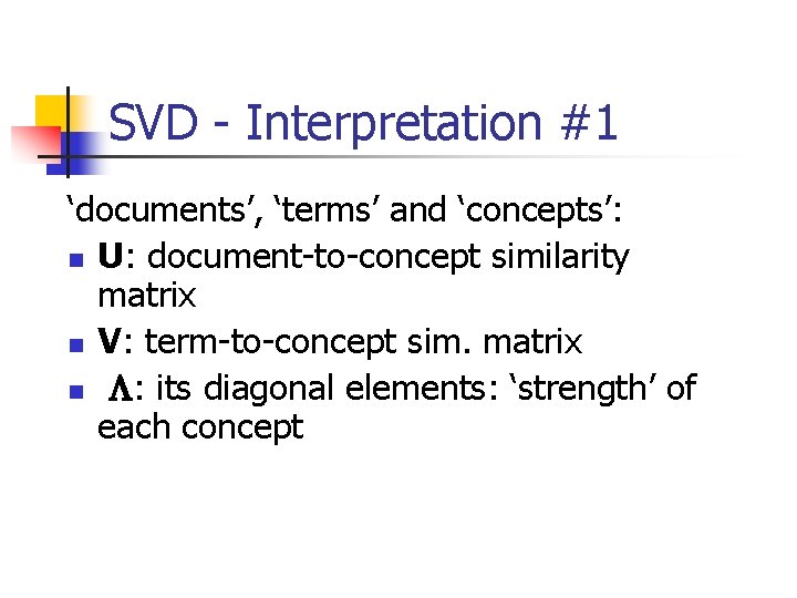
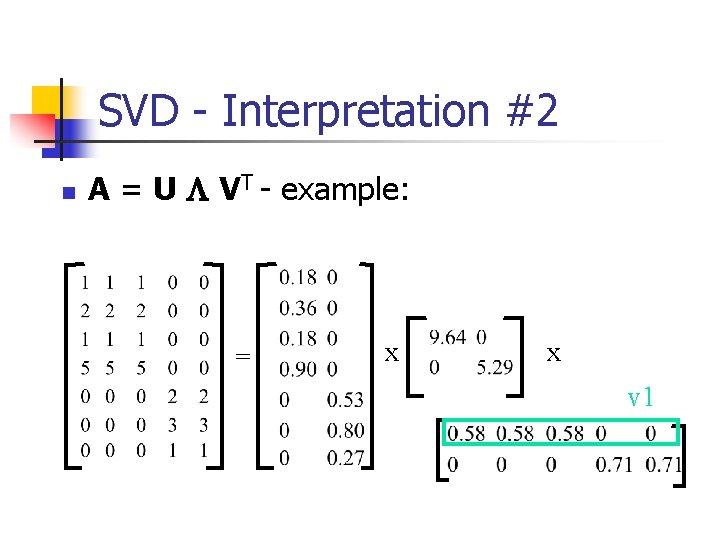
SVD - Interpretation #1 ‘documents’, ‘terms’ and ‘concepts’: n U: document-to-concept similarity matrix n V: term-to-concept sim. matrix n L: its diagonal elements: ‘strength’ of each concept

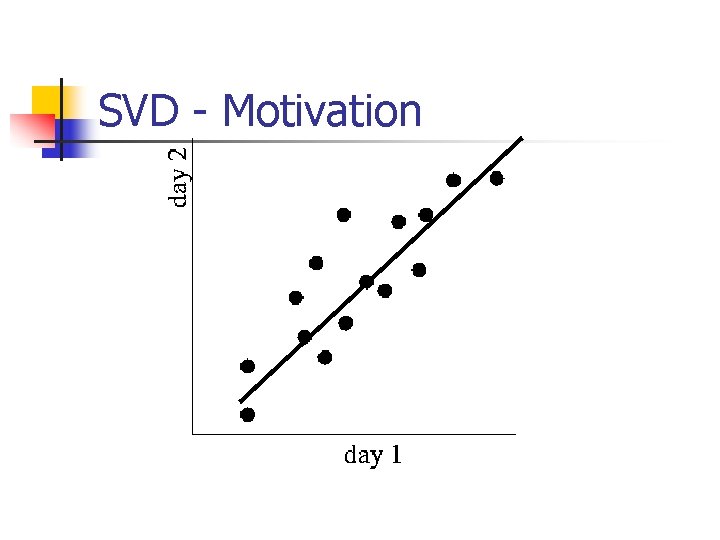
SVD - Interpretation #2 n best axis to project on: (‘best’ = min sum of squares of projection errors)

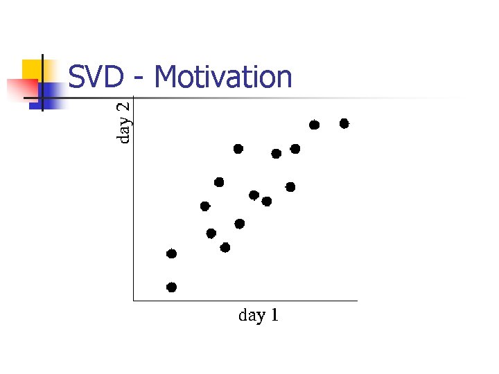
SVD - Motivation

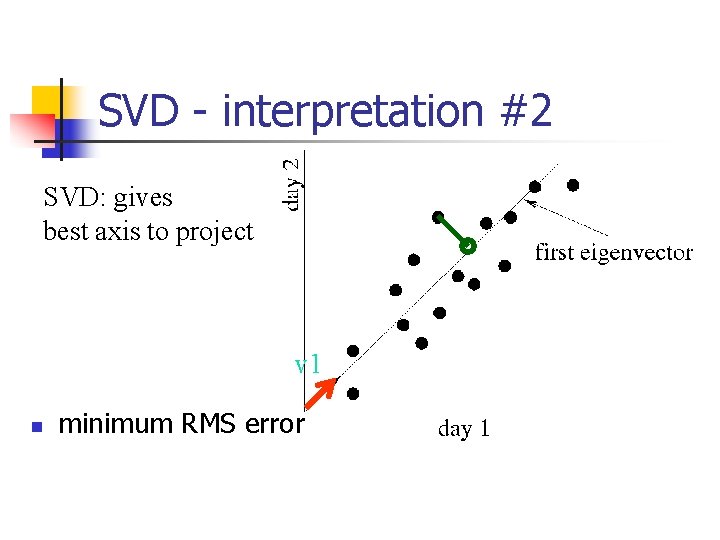
SVD - interpretation #2 SVD: gives best axis to project v 1 n minimum RMS error

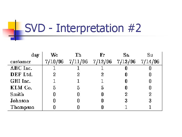
SVD - Interpretation #2

SVD - Interpretation #2 n A = U L VT - example: = x x v 1

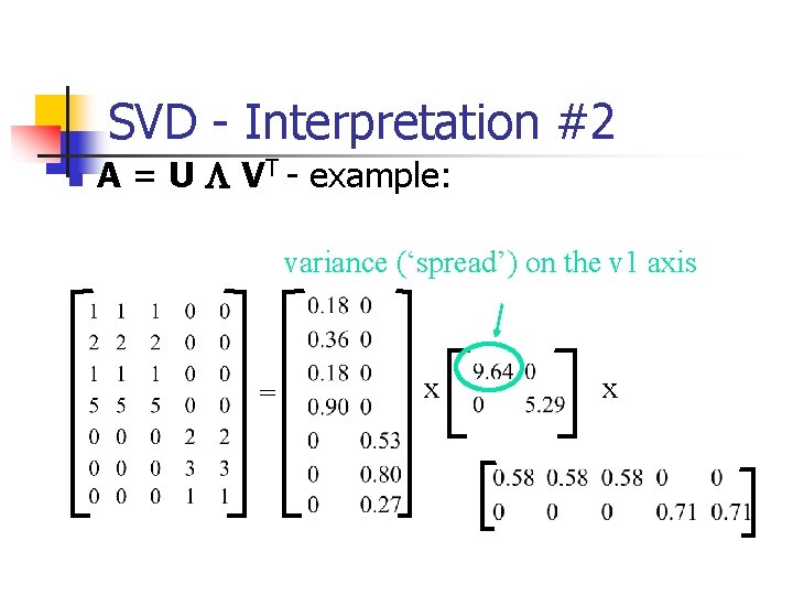
SVD - Interpretation #2 n A = U L VT - example: variance (‘spread’) on the v 1 axis = x x

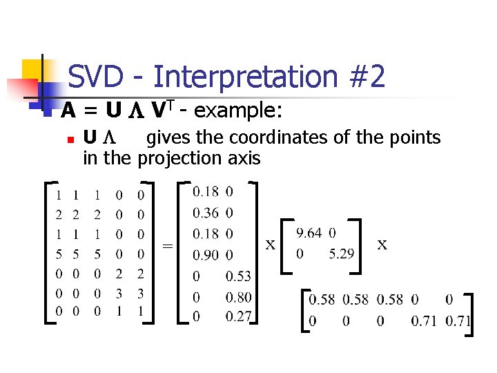
SVD - Interpretation #2 n A = U L VT - example: n UL gives the coordinates of the points in the projection axis = x x

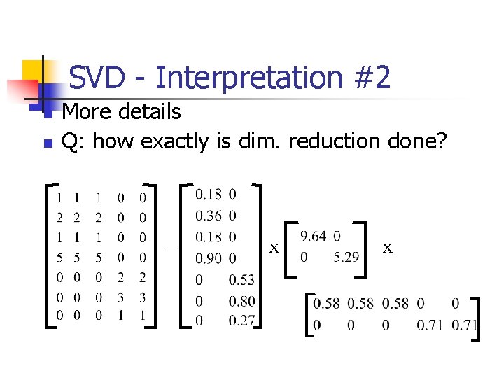
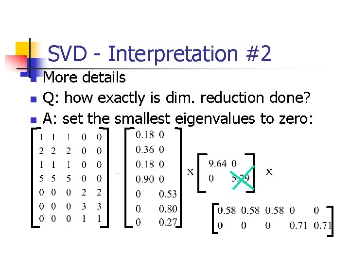
SVD - Interpretation #2 n n More details Q: how exactly is dim. reduction done? = x x

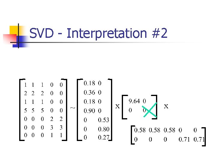
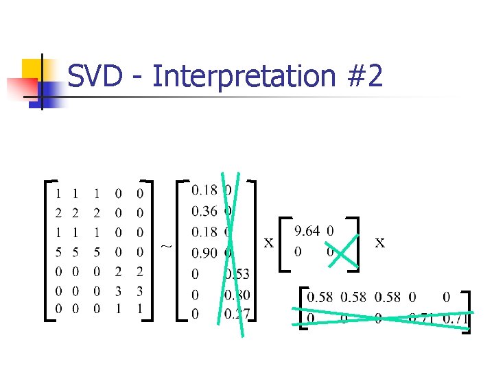
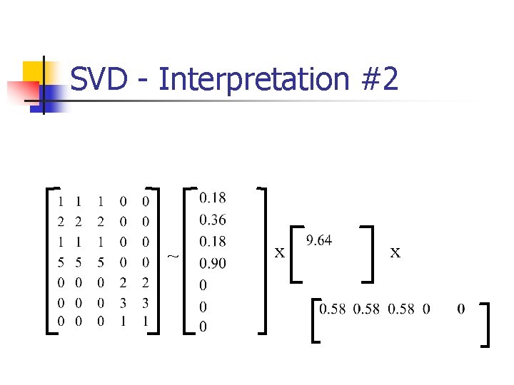
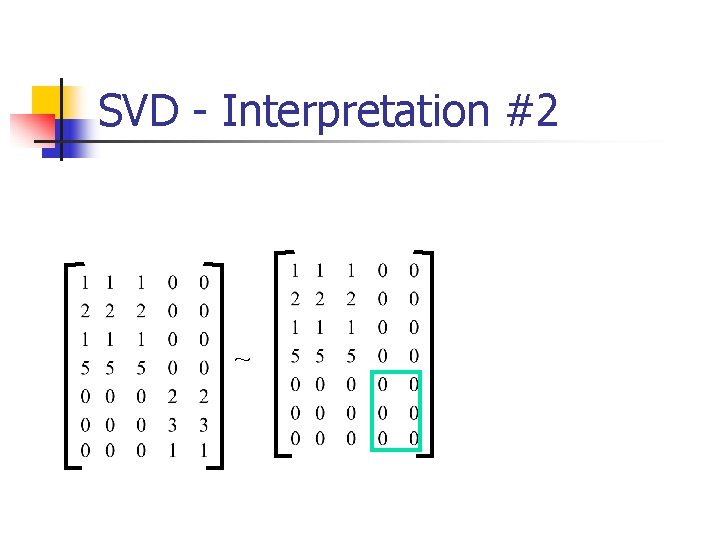
SVD - Interpretation #2 n n n More details Q: how exactly is dim. reduction done? A: set the smallest eigenvalues to zero: = x x

SVD - Interpretation #2 ~ x x

SVD - Interpretation #2 ~ x x

SVD - Interpretation #2 ~ x x

SVD - Interpretation #2 ~

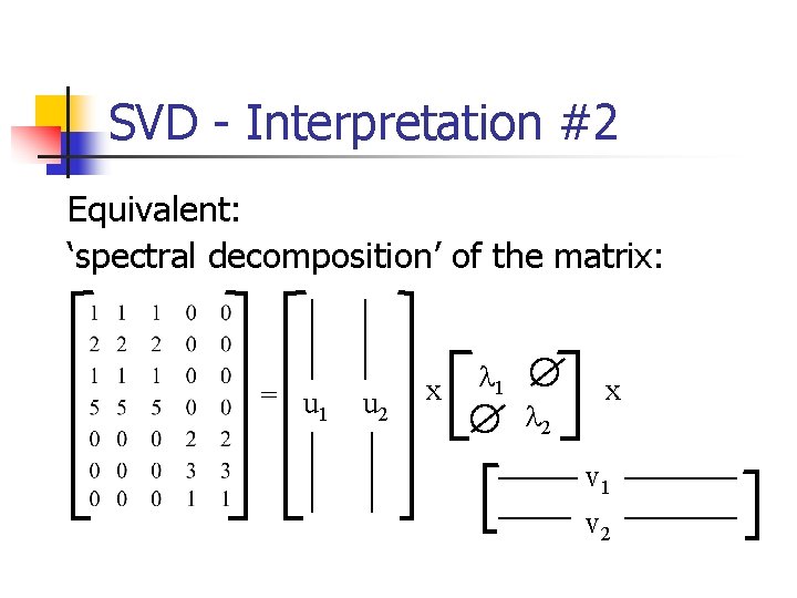
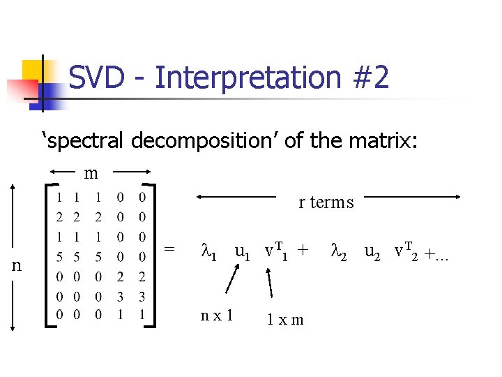
SVD - Interpretation #2 Equivalent: ‘spectral decomposition’ of the matrix: = x x

SVD - Interpretation #2 Equivalent: ‘spectral decomposition’ of the matrix: = u 1 u 2 x l 1 l 2 x v 1 v 2

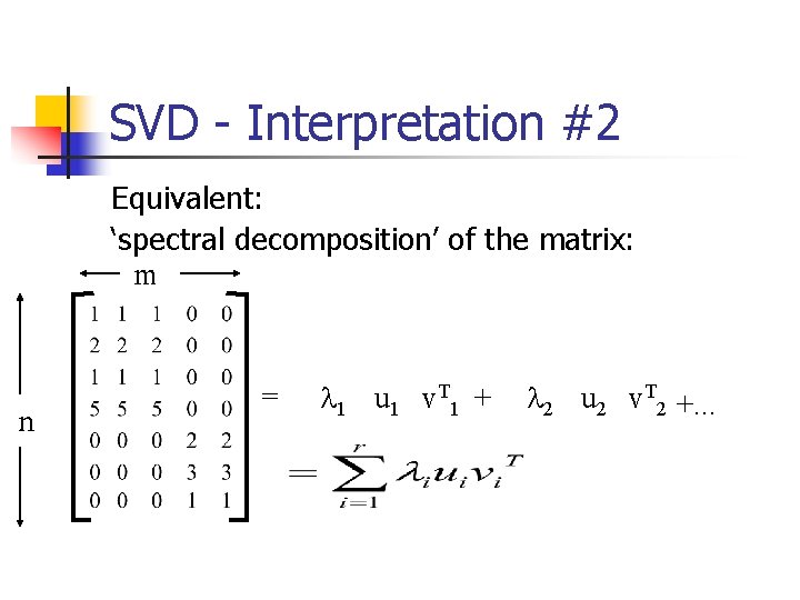
SVD - Interpretation #2 Equivalent: ‘spectral decomposition’ of the matrix: m n = l 1 u 1 v. T 1 + l 2 u 2 v. T 2 +. . .

SVD - Interpretation #2 ‘spectral decomposition’ of the matrix: m r terms n = l 1 u 1 v. T 1 + nx 1 1 xm l 2 u 2 v. T 2 +. . .

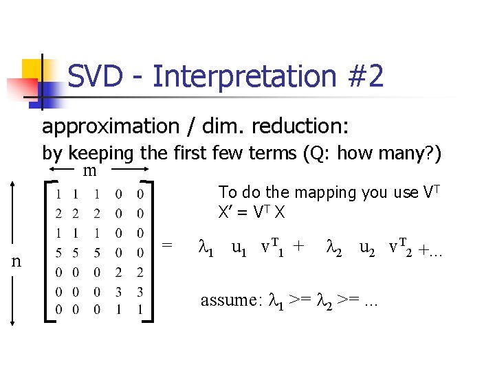
SVD - Interpretation #2 approximation / dim. reduction: by keeping the first few terms (Q: how many? ) m To do the mapping you use VT X’ = VT X n = l 1 u 1 v. T 1 + l 2 u 2 v. T 2 +. . . assume: l 1 >= l 2 >=. . .

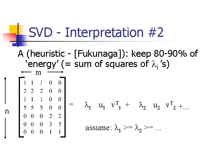
SVD - Interpretation #2 A (heuristic - [Fukunaga]): keep 80 -90% of ‘energy’ (= sum of squares of li ’s) m n = l 1 u 1 v. T 1 + l 2 u 2 v. T 2 +. . . assume: l 1 >= l 2 >=. . .

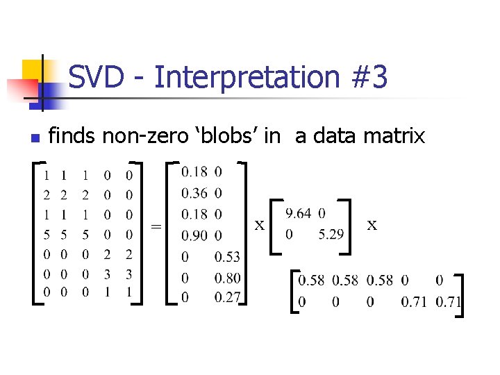
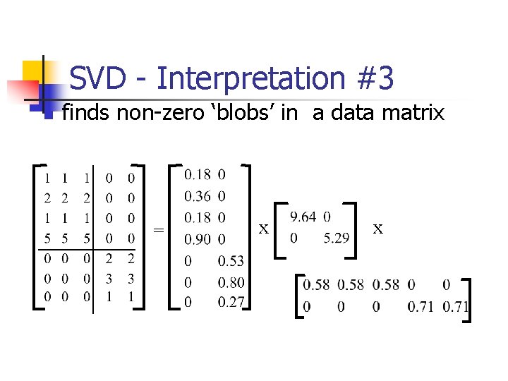
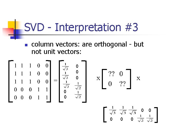
SVD - Interpretation #3 n finds non-zero ‘blobs’ in a data matrix = x x

SVD - Interpretation #3 n finds non-zero ‘blobs’ in a data matrix = x x

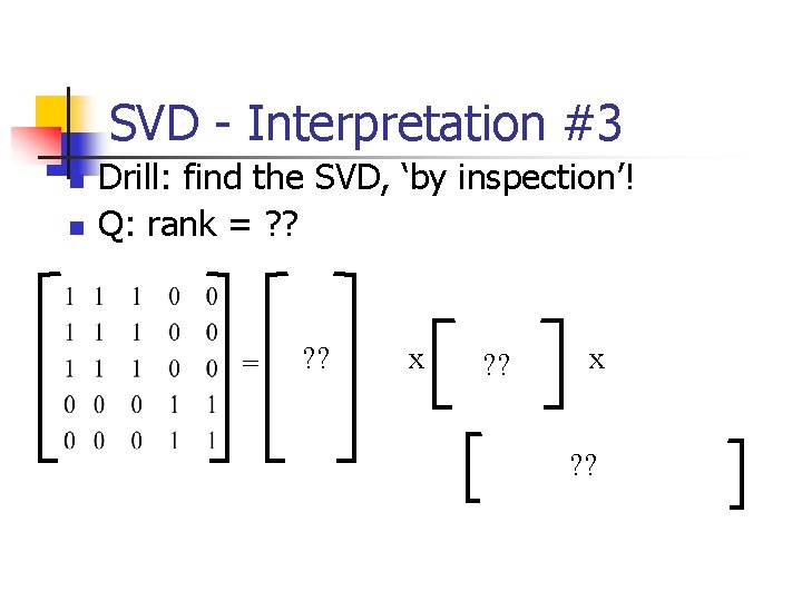
SVD - Interpretation #3 n n Drill: find the SVD, ‘by inspection’! Q: rank = ? ? x ? ?

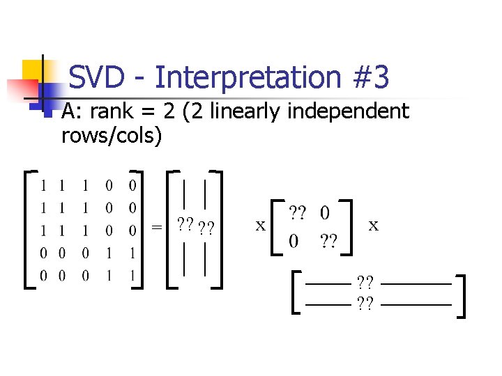
SVD - Interpretation #3 n A: rank = 2 (2 linearly independent rows/cols) = ? ? x x ? ?

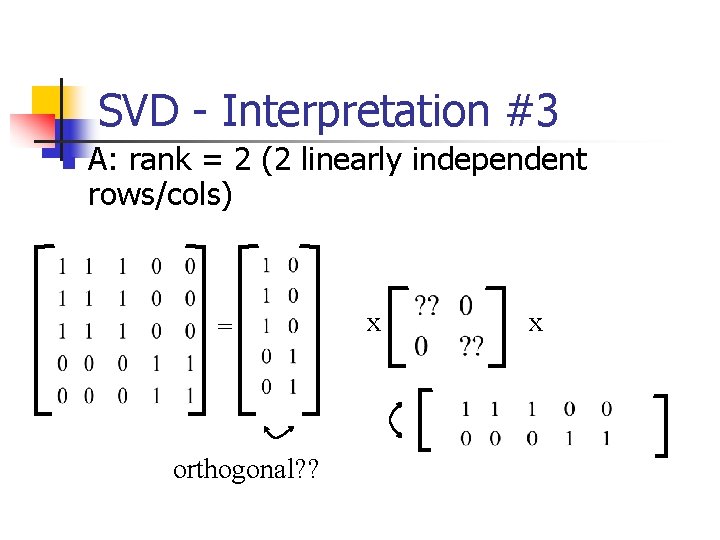
SVD - Interpretation #3 n A: rank = 2 (2 linearly independent rows/cols) = orthogonal? ? x x

SVD - Interpretation #3 n column vectors: are orthogonal - but not unit vectors: 0 0 0 = x x 0 0 0 0

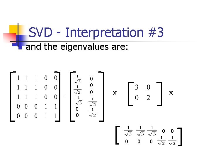
SVD - Interpretation #3 n and the eigenvalues are: 0 0 0 = x x 0 0 0 0

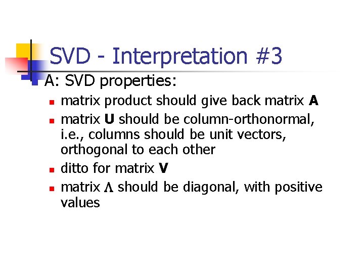
SVD - Interpretation #3 n A: SVD properties: n n matrix product should give back matrix A matrix U should be column-orthonormal, i. e. , columns should be unit vectors, orthogonal to each other ditto for matrix V matrix L should be diagonal, with positive values

SVD - Complexity n n n O( n * m) or O( n * m) (whichever is less) less work, if we just want eigenvalues or if we want first k eigenvectors or if the matrix is sparse [Berry] Implemented: in any linear algebra package (LINPACK, matlab, Splus, mathematica. . . )

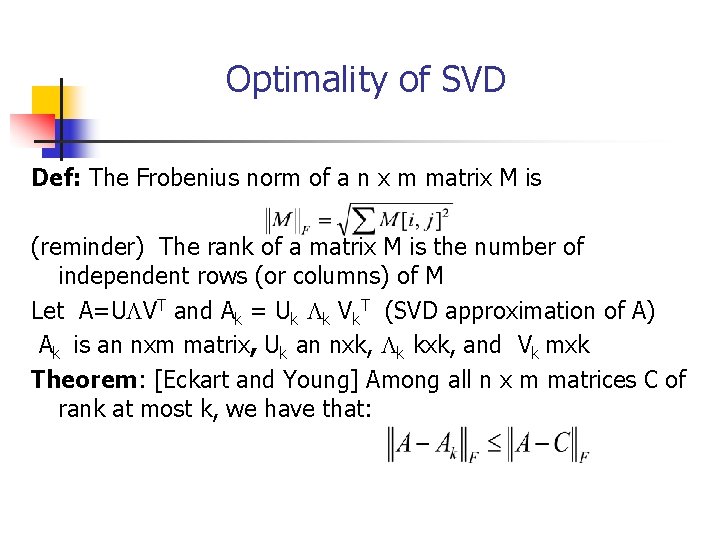
Optimality of SVD Def: The Frobenius norm of a n x m matrix M is (reminder) The rank of a matrix M is the number of independent rows (or columns) of M Let A=ULVT and Ak = Uk Lk Vk. T (SVD approximation of A) Ak is an nxm matrix, Uk an nxk, Lk kxk, and Vk mxk Theorem: [Eckart and Young] Among all n x m matrices C of rank at most k, we have that:

Kleinberg’s Algorithm n Main idea: In many cases, when you search the web using some terms, the most relevant pages may not contain this term (or contain the term only a few times) n n n Harvard : www. harvard. edu Search Engines: yahoo, google, altavista Authorities and hubs

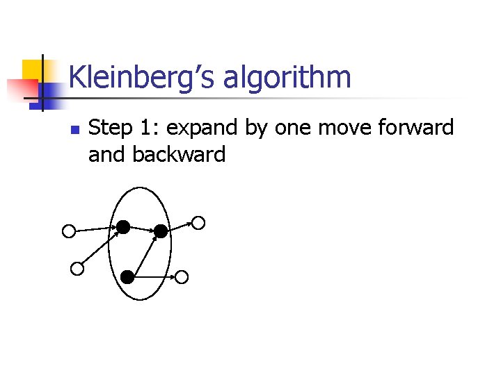
Kleinberg’s algorithm n n Problem dfn: given the web and a query find the most ‘authoritative’ web pages for this query Step 0: find all pages containing the query terms (root set) Step 1: expand by one move forward and backward (base set)

Kleinberg’s algorithm n Step 1: expand by one move forward and backward

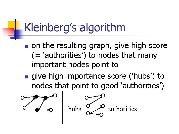
Kleinberg’s algorithm n n on the resulting graph, give high score (= ‘authorities’) to nodes that many important nodes point to give high importance score (‘hubs’) to nodes that point to good ‘authorities’) hubs authorities

Kleinberg’s algorithm observations n recursive definition! n each node (say, ‘i’-th node) has both an authoritativeness score ai and a hubness score hi

Kleinberg’s algorithm Let E be the set of edges and A be the adjacency matrix: the (i, j) is 1 if the edge from i to j exists Let h and a be [n x 1] vectors with the ‘hubness’ and ‘authoritativiness’ scores. Then:

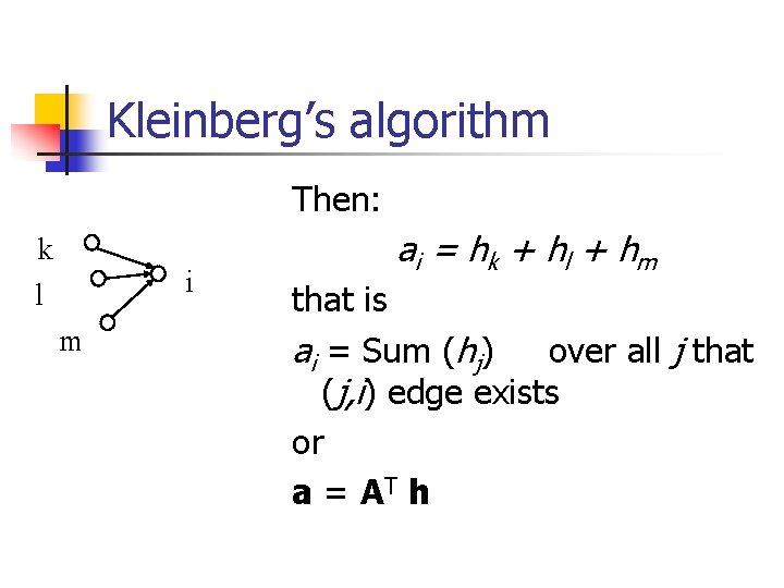
Kleinberg’s algorithm Then: k l i m a i = hk + h l + hm that is ai = Sum (hj) over all j that (j, i) edge exists or a = AT h

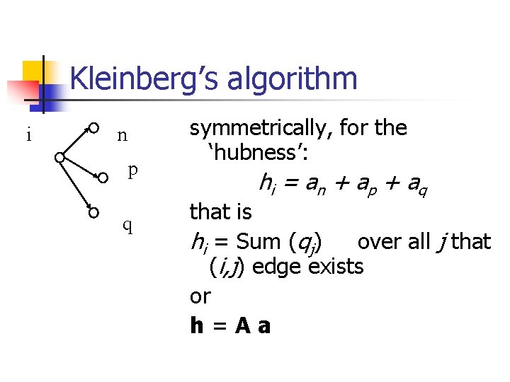
Kleinberg’s algorithm i n p q symmetrically, for the ‘hubness’: hi = a n + a p + a q that is hi = Sum (qj) over all j that (i, j) edge exists or h=Aa

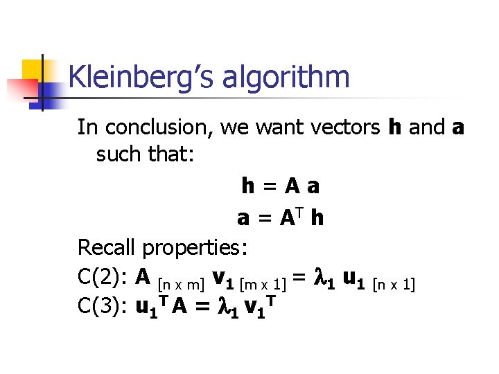
Kleinberg’s algorithm In conclusion, we want vectors h and a such that: h=Aa a = AT h Recall properties: C(2): A [n x m] v 1 [m x 1] = l 1 u 1 [n x 1] C(3): u 1 T A = l 1 v 1 T

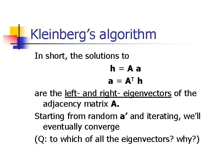
Kleinberg’s algorithm In short, the solutions to h=Aa a = AT h are the left- and right- eigenvectors of the adjacency matrix A. Starting from random a’ and iterating, we’ll eventually converge (Q: to which of all the eigenvectors? why? )

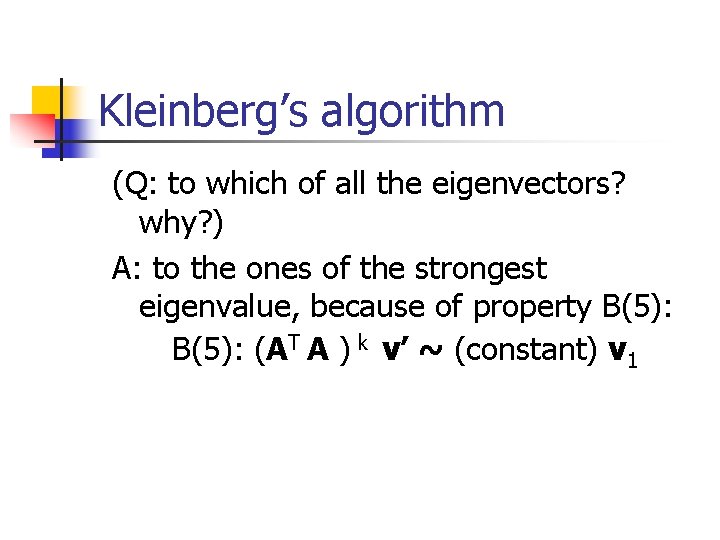
Kleinberg’s algorithm (Q: to which of all the eigenvectors? why? ) A: to the ones of the strongest eigenvalue, because of property B(5): (AT A ) k v’ ~ (constant) v 1

Kleinberg’s algorithm - results Eg. , for the query ‘java’: 0. 328 www. gamelan. com 0. 251 java. sun. com 0. 190 www. digitalfocus. com (“the java developer”)

Kleinberg’s algorithm - discussion n n ‘authority’ score can be used to find ‘similar pages’ to page p closely related to ‘citation analysis’, social networs / ‘small world’ phenomena

google/page-rank algorithm n n n closely related: The Web is a directed graph of connected nodes imagine a particle randomly moving along the edges (*) compute its steady-state probabilities. That gives the Page. Rank of each pages (the importance of this page) (*) with occasional random jumps

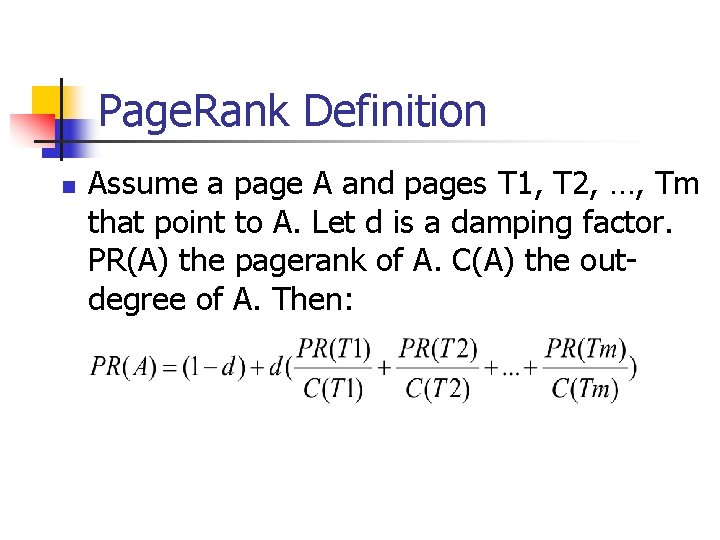
Page. Rank Definition n Assume a page A and pages T 1, T 2, …, Tm that point to A. Let d is a damping factor. PR(A) the pagerank of A. C(A) the outdegree of A. Then:

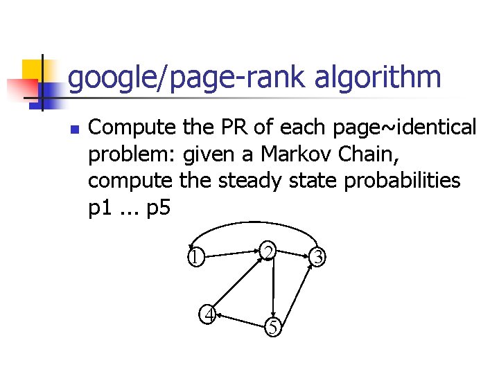
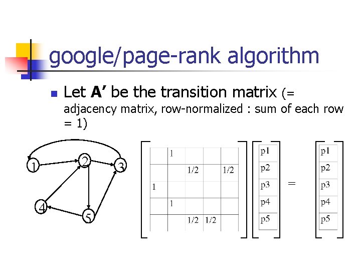
google/page-rank algorithm n Compute the PR of each page~identical problem: given a Markov Chain, compute the steady state probabilities p 1. . . p 5 2 1 4 5 3

Computing Page. Rank n n Iterative procedure Also, … navigate the web by randomly follow links or with prob p jump to a random page. Let A the adjacency matrix (n x n), di out-degree of page i Prob(Ai->Aj) = pn-1+(1 -p)di– 1 Aij A’[i, j] = Prob(Ai->Aj)

google/page-rank algorithm n Let A’ be the transition matrix (= adjacency matrix, row-normalized : sum of each row = 1) 2 1 3 = 4 5

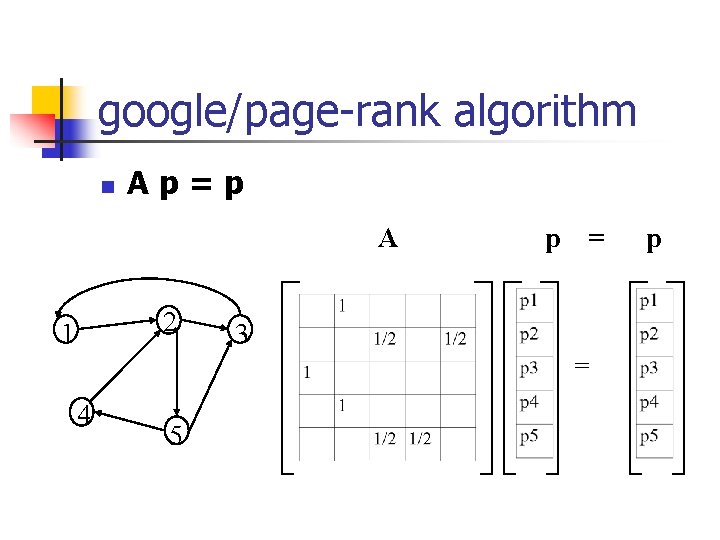
google/page-rank algorithm n Ap=p A 2 1 p = 3 = 4 5 p

google/page-rank algorithm n n Ap=p thus, p is the eigenvector that corresponds to the highest eigenvalue (=1, since the matrix is row-normalized)

Kleinberg/google - conclusions SVD helps in graph analysis: hub/authority scores: strongest left- and right- eigenvectors of the adjacency matrix random walk on a graph: steady state probabilities are given by the strongest eigenvector of the transition matrix

Conclusions – so far n n n SVD: a valuable tool given a document-term matrix, it finds ‘concepts’ (LSI). . . and can reduce dimensionality (KL)

Conclusions cont’d n n . . . and can find fixed-points or steadystate probabilities (google/ Kleinberg/ Markov Chains). . . and can solve optimally over- and under-constraint linear systems (least squares)

References n n Brin, S. and L. Page (1998). Anatomy of a Large-Scale Hypertextual Web Search Engine. 7 th Intl World Wide Web Conf. J. Kleinberg. Authoritative sources in a hyperlinked environment. Proc. 9 th ACM-SIAM Symposium on Discrete Algorithms, 1998.

Embeddings n n Given a metric distance matrix D, embed the objects in a k-dimensional vector space using a mapping F such that n D(i, j) is close to D’(F(i), F(j)) Isometric mapping: n exact preservation of distance Contractive mapping: n D’(F(i), F(j)) <= D(i, j) d’ is some Lp measure

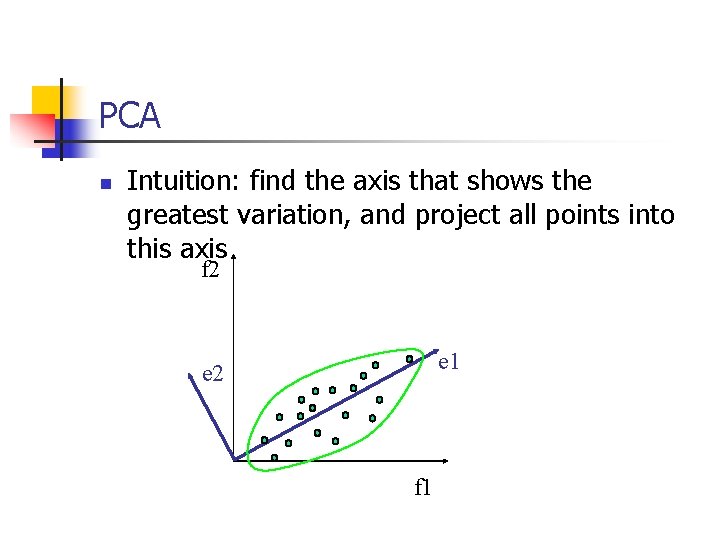
PCA n Intuition: find the axis that shows the greatest variation, and project all points into this axis f 2 e 1 e 2 f 1

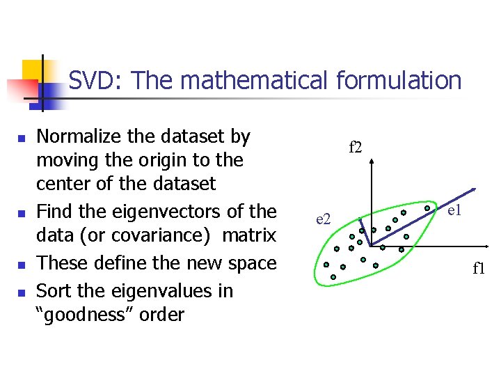
SVD: The mathematical formulation n n Normalize the dataset by moving the origin to the center of the dataset Find the eigenvectors of the data (or covariance) matrix These define the new space Sort the eigenvalues in “goodness” order f 2 e 1 f 1

SVD Cont’d n n Advantages: n Optimal dimensionality reduction (for linear projections) Disadvantages: n Computationally expensive… but can be improved with random sampling n Sensitive to outliers and non-linearities

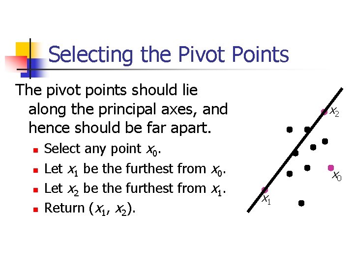
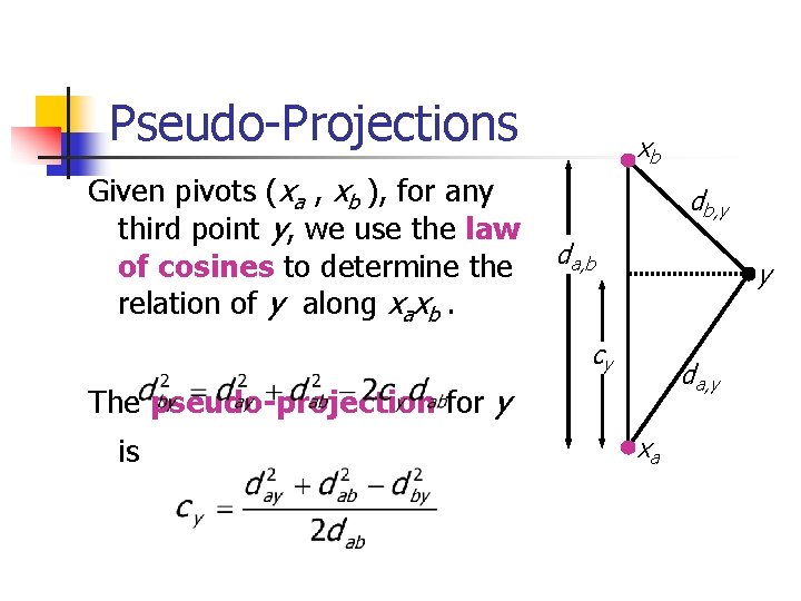
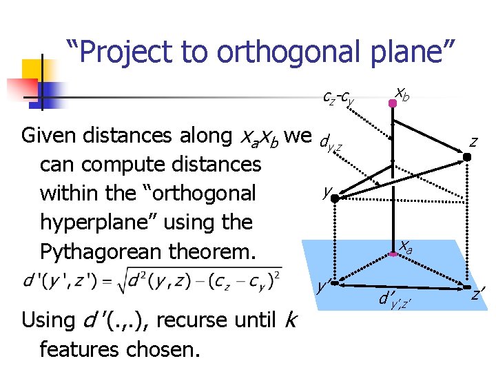
Fast. Map What if we have a finite metric space (X, d )? Faloutsos and Lin (1995) proposed Fast. Map as metric analogue to the KL-transform (PCA). Imagine that the points are in a Euclidean space. n Select two pivot points xa and xb that are far apart. n Compute a pseudo-projection of the remaining points along the “line” xaxb. n “Project” the points to an orthogonal subspace and recurse.

Selecting the Pivot Points The pivot points should lie along the principal axes, and hence should be far apart. x 2 Select any point x 0. Let x 1 be the furthest from x 0. Let x 2 be the furthest from x 1. Return (x 1, x 2). x 0 n n x 1

Pseudo-Projections Given pivots (xa , xb ), for any third point y, we use the law of cosines to determine the relation of y along xaxb. xb db, y da, b y cy da, y The pseudo-projection for y is xa

“Project to orthogonal plane” cz-cy Given distances along xaxb we dy, z can compute distances y within the “orthogonal hyperplane” using the Pythagorean theorem. y’ Using d ’(. , . ), recurse until k features chosen. xb z xa d’y’, z’ z’

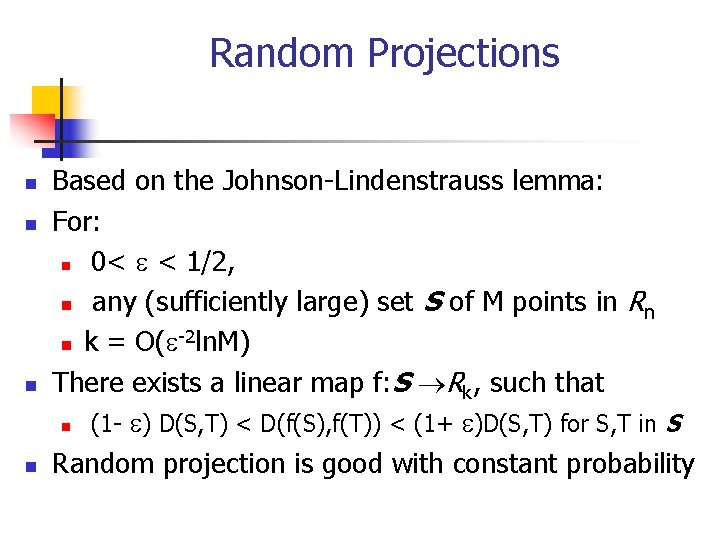
Random Projections n n Based on the Johnson-Lindenstrauss lemma: For: n 0< e < 1/2, n any (sufficiently large) set S of M points in R n -2 n k = O(e ln. M) There exists a linear map f: S Rk, such that n (1 - e) D(S, T) < D(f(S), f(T)) < (1+ e)D(S, T) for S, T in S Random projection is good with constant probability

Random Projection: Application n n Set k = O(e-2 ln. M) Select k random n-dimensional vectors n n n (an approach is to select k gaussian distributed vectors with variance 0 and mean value 1: N(1, 0) ) Project the original points into the k vectors. The resulting k-dimensional space approximately preserves the distances with high probability

Random Projection n A very useful technique, Especially when used in conjunction with another technique (for example SVD) Use Random projection to reduce the dimensionality from thousands to hundred, then apply SVD to reduce dimensionality farther