Dimensionality reduction Usman Roshan Dimensionality reduction What is

Dimensionality reduction Usman Roshan

Dimensionality reduction • What is dimensionality reduction? – Compress high dimensional data into lower dimensions • How do we achieve this? – PCA (unsupervised): We find a vector w of length 1 such that the variance of the projected data onto w is maximized. – Binary classification (supervised): Find a vector w that maximizes ratio (Fisher) or difference (MMC) of means and variances of the two classes.

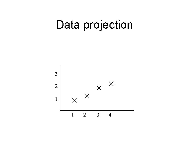
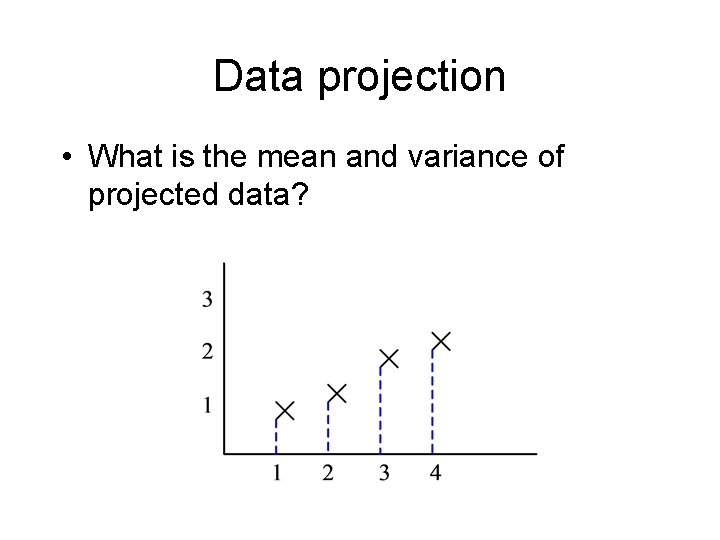
Data projection

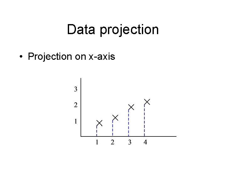
Data projection • Projection on x-axis

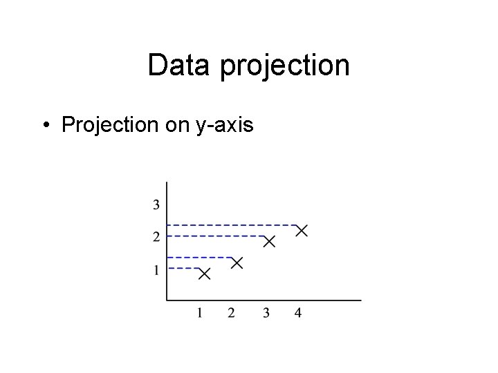
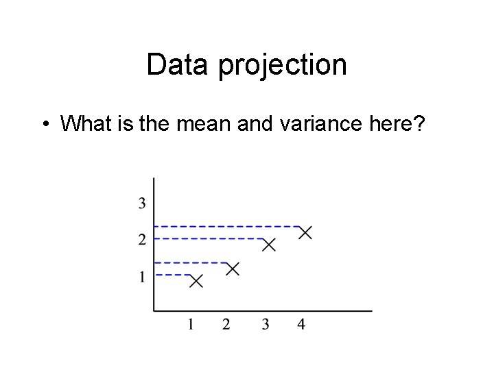
Data projection • Projection on y-axis

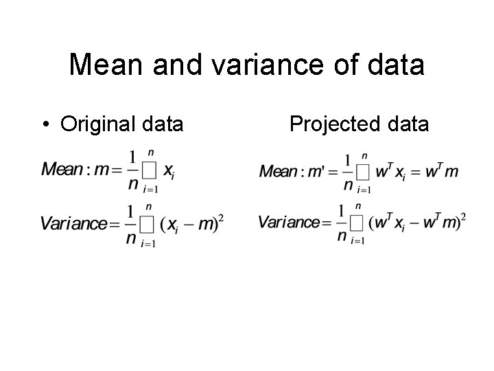
Mean and variance of data • Original data Projected data

Data projection • What is the mean and variance of projected data?

Data projection • What is the mean and variance here?

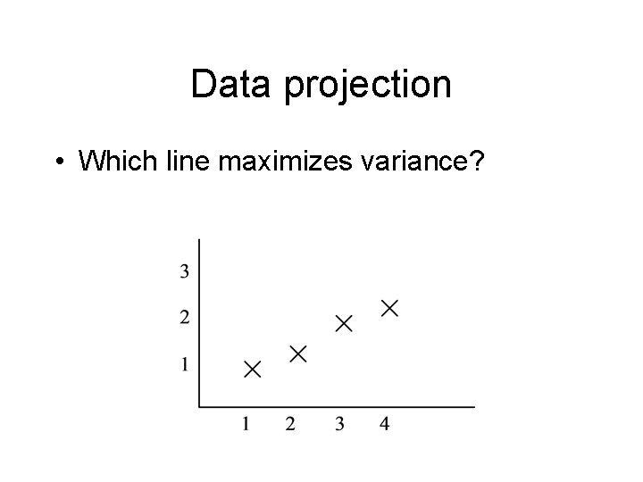
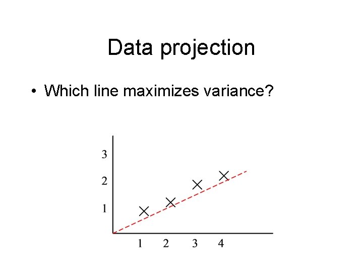
Data projection • Which line maximizes variance?

Data projection • Which line maximizes variance?

Principal component analysis • Find vector w of length 1 that maximizes variance of projected data

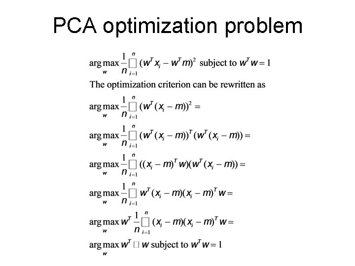
PCA optimization problem

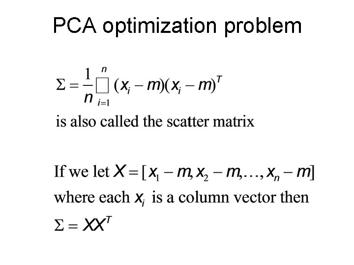
PCA optimization problem

PCA solution • Using Lagrange multipliers we can show that w is given by the largest eigenvector of ∑. • With this we can compress all the vectors xi into w. Txi • Does this help? Before looking at examples, what if we want to compute a second projection u. Txi such that w. Tu=0 and u. Tu=1? • It turns out that u is given by the second largest eigenvector of ∑.

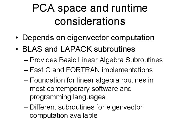
PCA space and runtime considerations • Depends on eigenvector computation • BLAS and LAPACK subroutines – Provides Basic Linear Algebra Subroutines. – Fast C and FORTRAN implementations. – Foundation for linear algebra routines in most contemporary software and programming languages. – Different subroutines for eigenvector computation available

PCA space and runtime considerations • Eigenvector computation requires quadratic space in number of columns • Poses a problem for high dimensional data • Instead we can use the Singular Value Decomposition

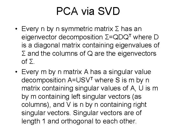
PCA via SVD • Every n by n symmetric matrix Σ has an eigenvector decomposition Σ=QDQT where D is a diagonal matrix containing eigenvalues of Σ and the columns of Q are the eigenvectors of Σ. • Every m by n matrix A has a singular value decomposition A=USVT where S is m by n matrix containing singular values of A, U is m by m containing left singular vectors (as columns), and V is n by n containing right singular vectors. Singular vectors are of length 1 and orthogonal to each other.

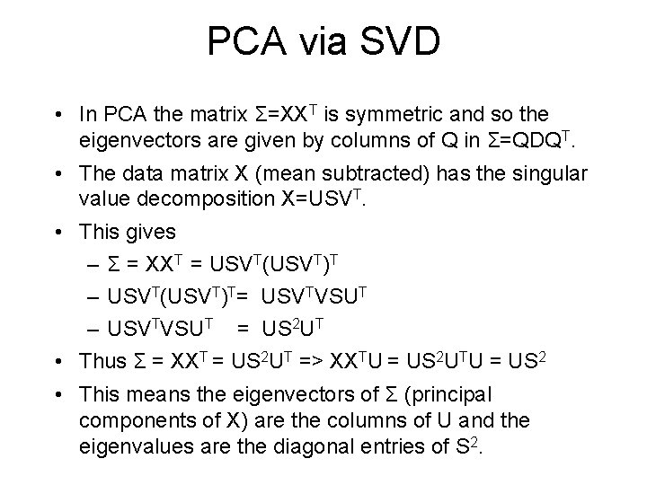
PCA via SVD • In PCA the matrix Σ=XXT is symmetric and so the eigenvectors are given by columns of Q in Σ=QDQT. • The data matrix X (mean subtracted) has the singular value decomposition X=USVT. • This gives – Σ = XXT = USVT(USVT)T – USVT(USVT)T= USVTVSUT – USVTVSUT = US 2 UT • Thus Σ = XXT = US 2 UT => XXTU = US 2 UTU = US 2 • This means the eigenvectors of Σ (principal components of X) are the columns of U and the eigenvalues are the diagonal entries of S 2.

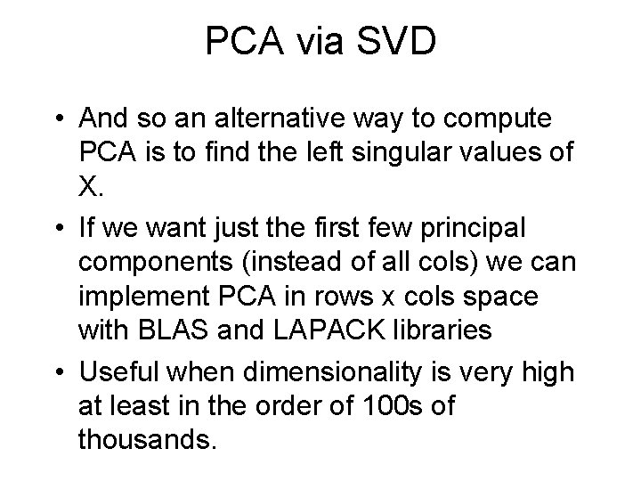
PCA via SVD • And so an alternative way to compute PCA is to find the left singular values of X. • If we want just the first few principal components (instead of all cols) we can implement PCA in rows x cols space with BLAS and LAPACK libraries • Useful when dimensionality is very high at least in the order of 100 s of thousands.

PCA on genomic population data • 45 Japanese and 45 Han Chinese from the International Hap. Map Project • PCA applied on 1. 7 million SNPs Taken from “PCA-Correlated SNPs for Structure Identification in Worldwide Human Populations” by Paschou et. al. in PLo. S Genetics 2007

PCA on breast cancer data

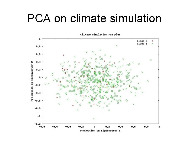
PCA on climate simulation

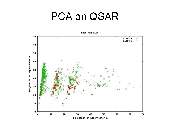
PCA on QSAR

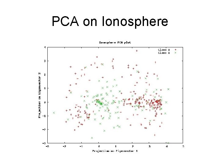
PCA on Ionosphere

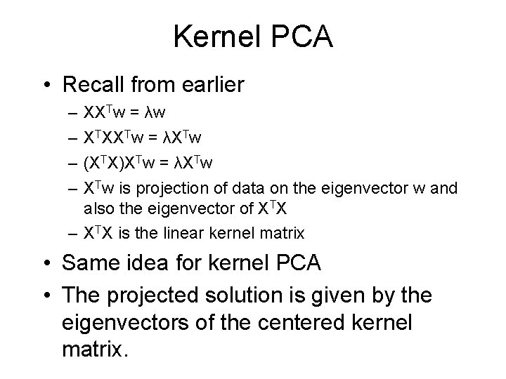
Kernel PCA • Main idea of kernel version – – XXTw = λw XTXXTw = λXTw (XTX)XTw = λXTw is projection of data on the eigenvector w and also the eigenvector of XTX • This is also another way to compute projections in space quadratic in number of rows but only gives projections.

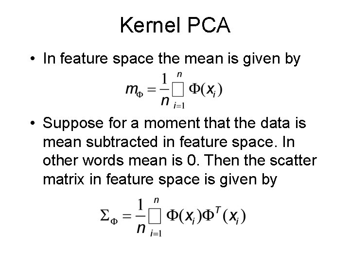
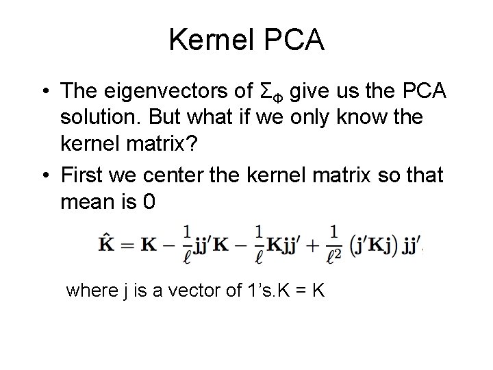
Kernel PCA • In feature space the mean is given by • Suppose for a moment that the data is mean subtracted in feature space. In other words mean is 0. Then the scatter matrix in feature space is given by

Kernel PCA • The eigenvectors of ΣΦ give us the PCA solution. But what if we only know the kernel matrix? • First we center the kernel matrix so that mean is 0 where j is a vector of 1’s. K = K

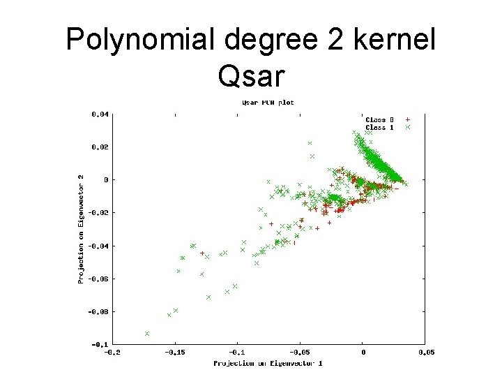
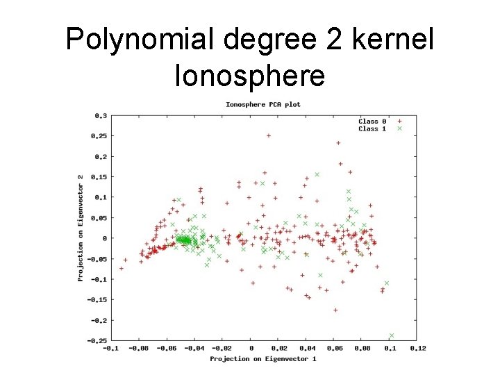
Kernel PCA • Recall from earlier – – XXTw = λw XTXXTw = λXTw (XTX)XTw = λXTw is projection of data on the eigenvector w and also the eigenvector of XTX – XTX is the linear kernel matrix • Same idea for kernel PCA • The projected solution is given by the eigenvectors of the centered kernel matrix.

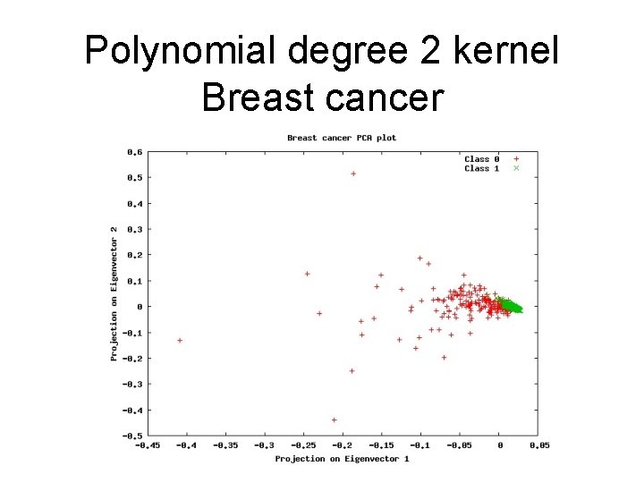
Polynomial degree 2 kernel Breast cancer

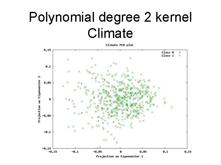
Polynomial degree 2 kernel Climate

Polynomial degree 2 kernel Qsar

Polynomial degree 2 kernel Ionosphere

Random projections • What if we projected our data onto random vectors instead of PCA or LDA? • Turns out that random projections preserve distances upto a certain error

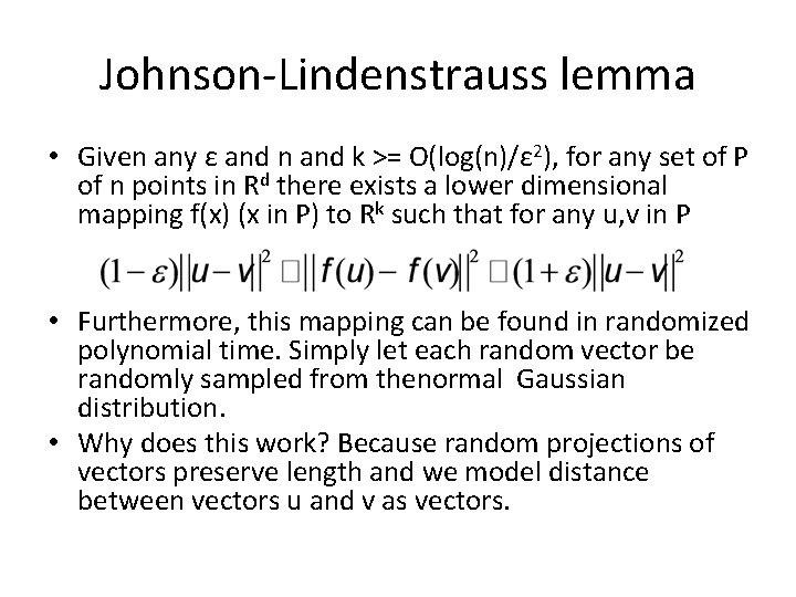
Johnson-Lindenstrauss lemma • Given any ε and n and k >= O(log(n)/ε 2), for any set of P of n points in Rd there exists a lower dimensional mapping f(x) (x in P) to Rk such that for any u, v in P • Furthermore, this mapping can be found in randomized polynomial time. Simply let each random vector be randomly sampled from thenormal Gaussian distribution. • Why does this work? Because random projections of vectors preserve length and we model distance between vectors u and v as vectors.