Dimensionality reduction Dimensionality Reduction Feature vectors have often

Dimensionality reduction

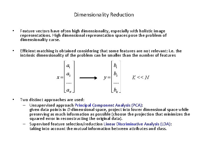
Dimensionality Reduction • Feature vectors have often high dimensionality, especially with holistic image representations. High dimensional representation spaces pose the problem of dimensionality curse. • Efficient matching is obtained considering that some features are not relevant: i. e. the intrinsic dimensionality of the problem can be smaller than the number of features K << N • Two distinct approaches are used: – Unsupervised approach Principal Component Analysis (PCA): given data points in D-dimensional space, project into lower dimensional space while preserving as much information as possible (choose the projection that minimizes the squared error in reconstructing the original data). – Supervised feature selection/reduction Linear Discriminative Analysis (LDA): taking into account the mutual information between attributes and class.

Principal Component Analysis • Principal Component Analysis (PCA) aims to reduce the dimensionality of the data while retaining as much as possible of the variation in the original dataset. Wish to summarize the underlying variancecovariance structure of a large set of variables through a few linear combinations of these variables. • Uses: – Data Visualization: how many unique “sub-sets” are in the sample? – Data Reduction: how are they similar / different? – Data Classification: what are the underlying factors that influence the samples? – Trend Analysis: which temporal trends are (anti)correlated? – Factor Analysis: which measurements are needed to differentiate? – Noise Reduction: which “sub-set” does this new sample rightfully belong?

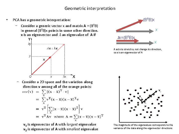
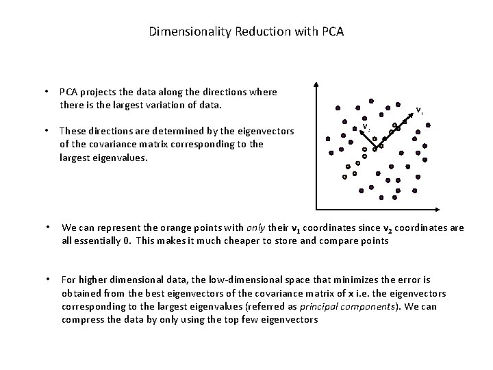
Geometric interpretation • PCA has a geometric interpretation: − Consider a generic vector x and matrix A = (BTB) In general (BTB)x points in some other direction. x is an eigenvector and l an eigenvalue of A if (BTB)x x lx=(BTB)x x A acts to stretch x, not change its direction, so x is an eigenvector of A − Consider a 2 D space and the variation along direction v among all of the orange points: v 1 is eigenvector of A with largest eigenvalue v 2 is eigenvector of A with smallest eigenvalue The magnitude of the eigenvalues corresponds to the variance of the data along the eigenvector directions.

Dimensionality Reduction with PCA • PCA projects the data along the directions where there is the largest variation of data. • These directions are determined by the eigenvectors of the covariance matrix corresponding to the largest eigenvalues. • We can represent the orange points with only their v 1 coordinates since v 2 coordinates are all essentially 0. This makes it much cheaper to store and compare points • For higher dimensional data, the low-dimensional space that minimizes the error is obtained from the best eigenvectors of the covariance matrix of x i. e. the eigenvectors corresponding to the largest eigenvalues (referred as principal components). We can compress the data by only using the top few eigenvectors

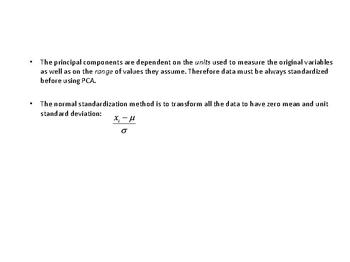
• The principal components are dependent on the units used to measure the original variables as well as on the range of values they assume. Therefore data must be always standardized before using PCA. • The normal standardization method is to transform all the data to have zero mean and unit standard deviation:

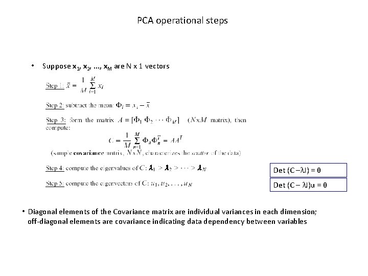
PCA operational steps • Suppose x 1, x 2, . . . , x. M are N x 1 vectors Det (C –l. I) = 0 Det (C – l. I)u = 0 • Diagonal elements of the Covariance matrix are individual variances in each dimension; off-diagonal elements are covariance indicating data dependency between variables

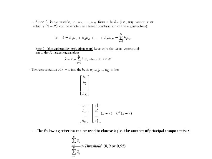
− The following criterion can be used to choose K (i. e. the number of principal components) :

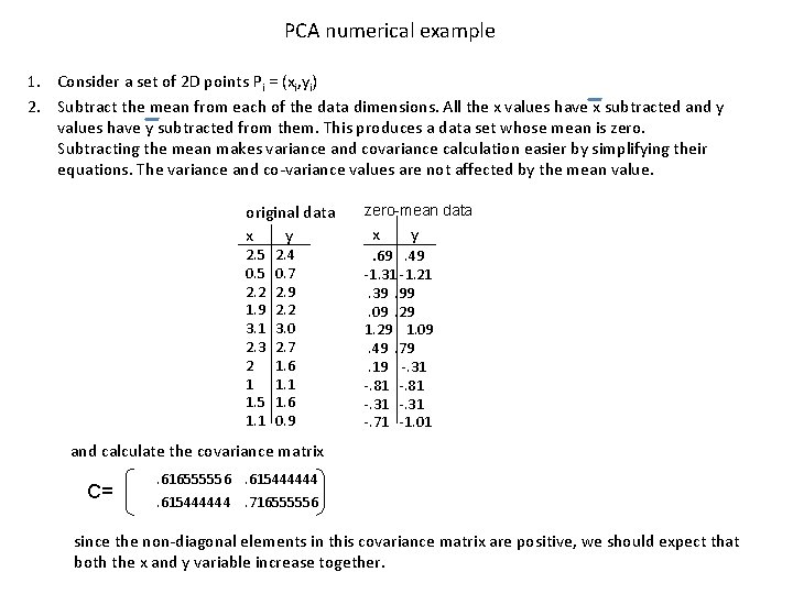
PCA numerical example 1. Consider a set of 2 D points Pi = (xi, yi) 2. Subtract the mean from each of the data dimensions. All the x values have x subtracted and y values have y subtracted from them. This produces a data set whose mean is zero. Subtracting the mean makes variance and covariance calculation easier by simplifying their equations. The variance and co-variance values are not affected by the mean value. original data x y 2. 5 0. 5 2. 2 1. 9 3. 1 2. 3 2 1 1. 5 1. 1 2. 4 0. 7 2. 9 2. 2 3. 0 2. 7 1. 6 1. 1 1. 6 0. 9 zero-mean data x y. 69. 49 -1. 31 -1. 21. 39. 99. 09. 29 1. 09. 49. 79. 19 -. 31 -. 81 -. 31 -. 71 -1. 01 and calculate the covariance matrix C= . 616555556. 615444444. 716555556 since the non-diagonal elements in this covariance matrix are positive, we should expect that both the x and y variable increase together.

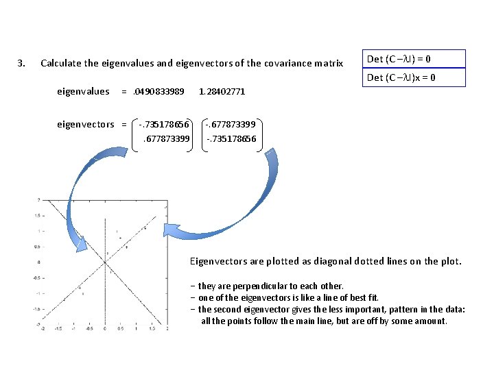
3. Calculate the eigenvalues and eigenvectors of the covariance matrix Det (C –l. I) = 0 Det (C –l. I)x = 0 eigenvalues =. 0490833989 eigenvectors = -. 735178656. 677873399 1. 28402771 -. 677873399 -. 735178656 Eigenvectors are plotted as diagonal dotted lines on the plot. − they are perpendicular to each other. − one of the eigenvectors is like a line of best fit. − the second eigenvector gives the less important, pattern in the data: all the points follow the main line, but are off by some amount.

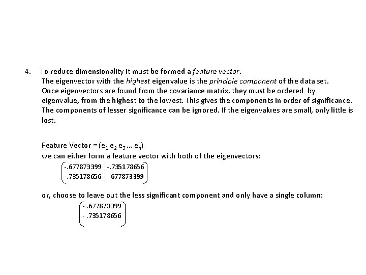
4. To reduce dimensionality it must be formed a feature vector. The eigenvector with the highest eigenvalue is the principle component of the data set. Once eigenvectors are found from the covariance matrix, they must be ordered by eigenvalue, from the highest to the lowest. This gives the components in order of significance. The components of lesser significance can be ignored. If the eigenvalues are small, only little is lost. Feature Vector = (e 1 e 2 e 3 … en) we can either form a feature vector with both of the eigenvectors: -. 677873399 -. 735178656. 677873399 or, choose to leave out the less significant component and only have a single column: -. 677873399 -. 735178656

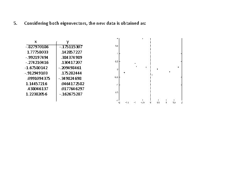
5. Considering both eigenvectors, the new data is obtained as: x -. 827970186 1. 77758033 -. 992197494 -. 274210416 -1. 67580142 -. 912949103. 0991094375 1. 14457216. 438046137 1. 22382056 y -. 175115307. 142857227. 384374989. 130417207 -. 209498461. 175282444 -. 349824698. 0464172582. 0177646297 -. 162675287

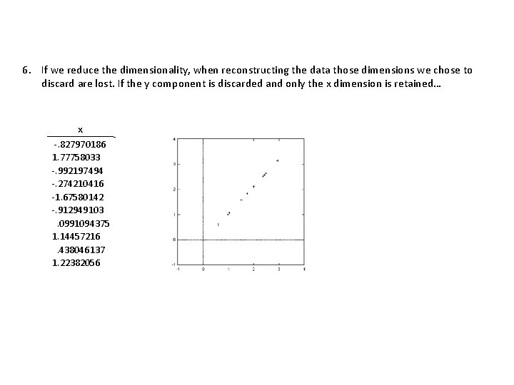
6. If we reduce the dimensionality, when reconstructing the data those dimensions we chose to discard are lost. If the y component is discarded and only the x dimension is retained… x -. 827970186 1. 77758033 -. 992197494 -. 274210416 -1. 67580142 -. 912949103. 0991094375 1. 14457216. 438046137 1. 22382056

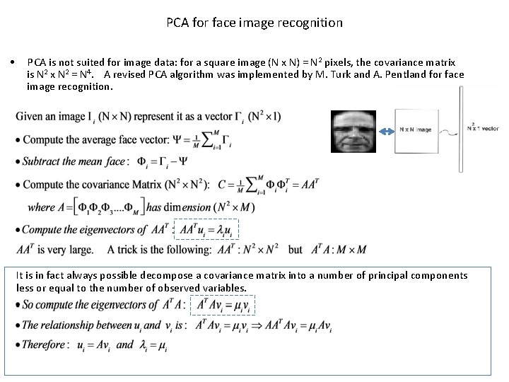
PCA for face image recognition • PCA is not suited for image data: for a square image (N x N) = N 2 pixels, the covariance matrix is N 2 x N 2 = N 4. A revised PCA algorithm was implemented by M. Turk and A. Pentland for face image recognition. It is in fact always possible decompose a covariance matrix into a number of principal components less or equal to the number of observed variables.

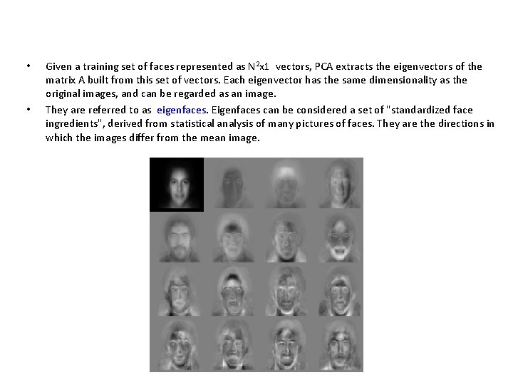
• • Given a training set of faces represented as N 2 x 1 vectors, PCA extracts the eigenvectors of the matrix A built from this set of vectors. Each eigenvector has the same dimensionality as the original images, and can be regarded as an image. They are referred to as eigenfaces. Eigenfaces can be considered a set of "standardized face ingredients", derived from statistical analysis of many pictures of faces. They are the directions in which the images differ from the mean image.

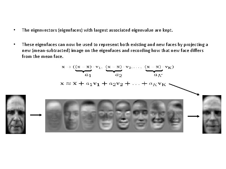
• The eigenvectors (eigenfaces) with largest associated eigenvalue are kept. • These eigenfaces can now be used to represent both existing and new faces by projecting a new (mean-subtracted) image on the eigenfaces and recording how that new face differs from the mean face.

• Computation of the covariance matrix is simplified (suppose 300 images of 100 x 100 pixels, that yelds a 10000 x 10000 covariance matrix. Eigenvalues are instead extracted from 300 x 300 covariance matrix). • In practical applications, most faces can be identified using a projection on between 100 and 150 eigenfaces, so that most of the eigenvectors can be discarded.

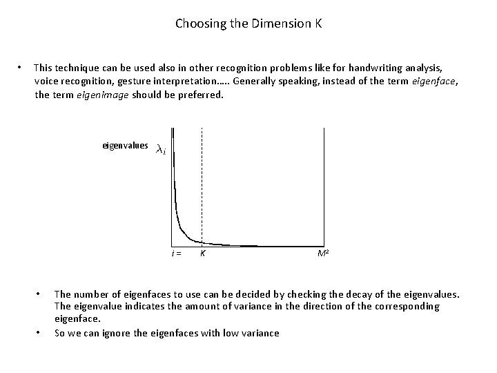
Choosing the Dimension K • This technique can be used also in other recognition problems like for handwriting analysis, voice recognition, gesture interpretation…. . Generally speaking, instead of the term eigenface, the term eigenimage should be preferred. eigenvalues i= • • K M 2 The number of eigenfaces to use can be decided by checking the decay of the eigenvalues. The eigenvalue indicates the amount of variance in the direction of the corresponding eigenface. So we can ignore the eigenfaces with low variance

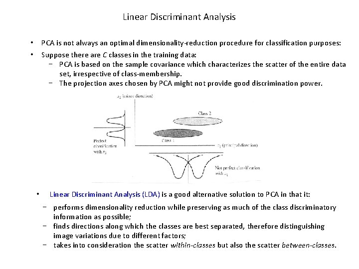
Linear Discriminant Analysis PCA is not always an optimal dimensionality-reduction procedure for classification purposes: Suppose there are C classes in the training data: − PCA is based on the sample covariance which characterizes the scatter of the entire data set, irrespective of class-membership. − The projection axes chosen by PCA might not provide good discrimination power. • • • Linear Discriminant Analysis (LDA) is a good alternative solution to PCA in that it: − performs dimensionality reduction while preserving as much of the class discriminatory information as possible; − finds directions along which the classes are best separated, therefore distinguishing image variations due to different factors; − takes into consideration the scatter within-classes but also the scatter between-classes.

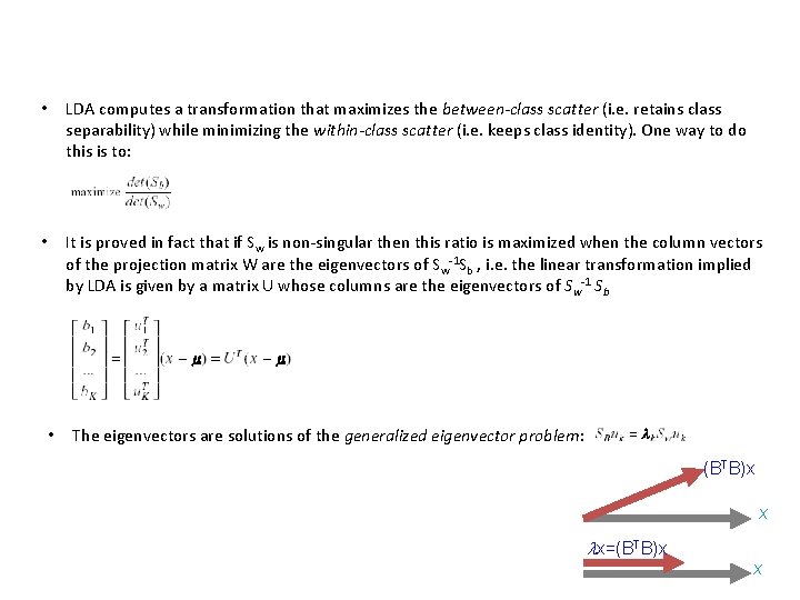
• LDA computes a transformation that maximizes the between-class scatter (i. e. retains class separability) while minimizing the within-class scatter (i. e. keeps class identity). One way to do this is to: • It is proved in fact that if Sw is non-singular then this ratio is maximized when the column vectors of the projection matrix W are the eigenvectors of Sw-1 Sb , i. e. the linear transformation implied by LDA is given by a matrix U whose columns are the eigenvectors of Sw-1 Sb • The eigenvectors are solutions of the generalized eigenvector problem: (BTB)x x lx=(BTB)x x

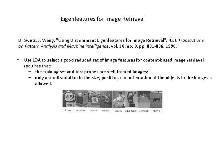
Eigenfeatures for Image Retrieval D. Swets, J. Weng, "Using Discriminant Eigenfeatures for Image Retrieval", IEEE Transactions on Pattern Analysis and Machine Intelligence, vol. 18, no. 8, pp. 831 -836, 1996. • Use LDA to select a good reduced set of image features for content-based image retrieval requires that: − the training set and test probes are well-framed images; − only a small variation in the size, position, and orientation of the objects in the images is allowed.

PCA versus LDA A. Martinez, A. Kak, "PCA versus LDA", IEEE Transactions on Pattern Analysis and Machine Intelligence, vol. 23, no. 2, pp. 228 -233, 2001. • Is LDA always better than PCA? − There has been a tendency in the computer vision community to prefer LDA over PCA, mainly because LDA deals directly with discrimination between classes while PCA does not pay attention to the underlying class structure. − However, when the training set is small, PCA can outperform LDA. − When the number of samples is large and representative for each class, LDA outperforms PCA.