Feature Reduction Algorithms What is feature reduction Feature

Feature Reduction Algorithms

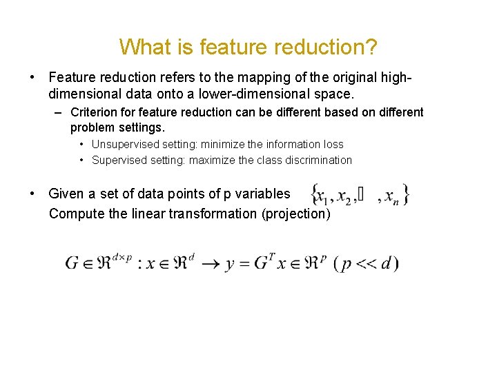
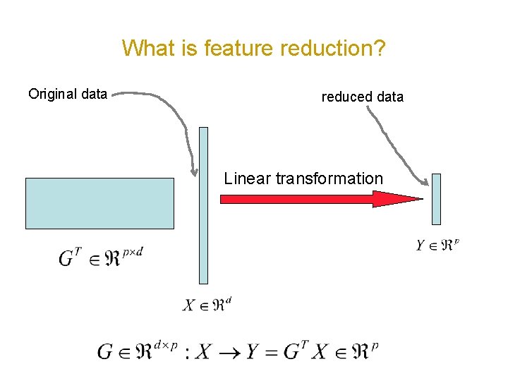
What is feature reduction? • Feature reduction refers to the mapping of the original highdimensional data onto a lower-dimensional space. – Criterion for feature reduction can be different based on different problem settings. • Unsupervised setting: minimize the information loss • Supervised setting: maximize the class discrimination • Given a set of data points of p variables Compute the linear transformation (projection)

What is feature reduction? Original data reduced data Linear transformation

Outline of lecture • What is feature reduction? • Why feature reduction? • Feature reduction algorithms – Principal Component Analysis (PCA) – Linear Discriminant Analysis (LDA)

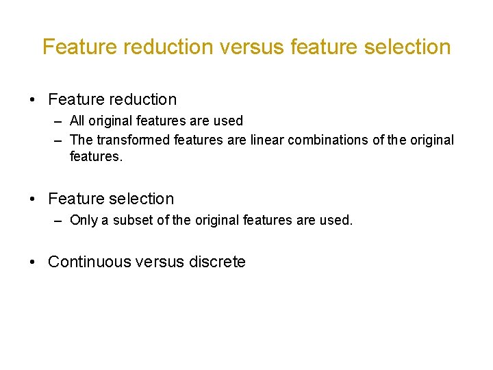
Feature reduction versus feature selection • Feature reduction – All original features are used – The transformed features are linear combinations of the original features. • Feature selection – Only a subset of the original features are used. • Continuous versus discrete

Outline of lecture • What is feature reduction? • Why feature reduction? • Feature reduction algorithms – Principal Component Analysis (PCA) – Linear Discriminant Analysis (LDA)

Why feature reduction? • Most machine learning and data mining techniques may not be effective for high-dimensional data – Curse of Dimensionality – Query accuracy and efficiency degrade rapidly as the dimension increases. • The intrinsic dimension may be small. – For example, the number of genes responsible for a certain type of disease may be small.

Why feature reduction? • Visualization: projection of high-dimensional data onto 2 D or 3 D. • Data compression: efficient storage and retrieval. • Noise removal: positive effect on query accuracy.

Applications of feature reduction • • • Face recognition Handwritten digit recognition Text mining Image retrieval Microarray data analysis Protein classification

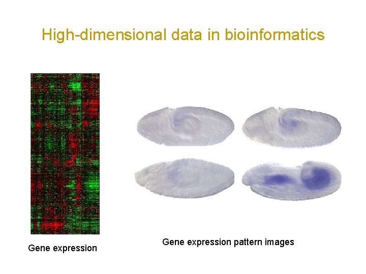
High-dimensional data in bioinformatics Gene expression pattern images

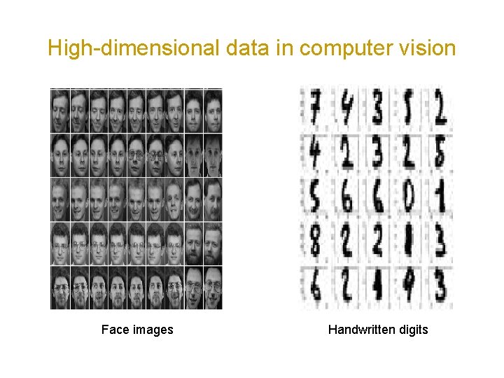
High-dimensional data in computer vision Face images Handwritten digits

Outline of lecture • What is feature reduction? • Why feature reduction? • Feature reduction algorithms – Principal Component Analysis (PCA) – Linear Discriminant Analysis (LDA)

What is Principal Component Analysis? • Principal component analysis (PCA) – Reduce the dimensionality of a data set by finding a new set of variables, smaller than the original set of variables – Retains most of the sample's information. – Useful for the compression and classification of data. • By information we mean the variation present in the sample, given by the correlations between the original variables. – The new variables, called principal components (PCs), are uncorrelated, and are ordered by the fraction of the total information each retains.

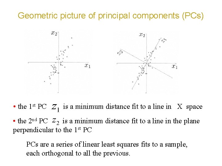
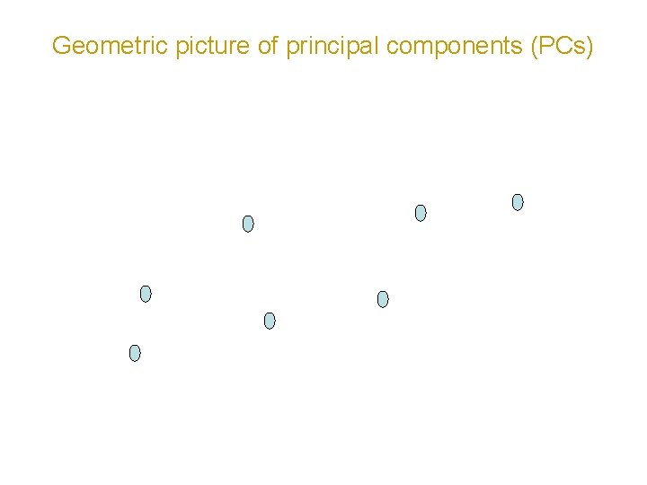
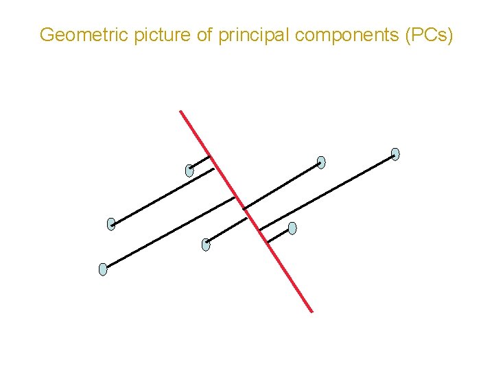
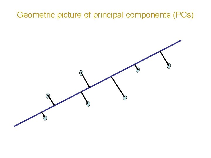
Geometric picture of principal components (PCs) • the 1 st PC is a minimum distance fit to a line in X space • the 2 nd PC is a minimum distance fit to a line in the plane perpendicular to the 1 st PC PCs are a series of linear least squares fits to a sample, each orthogonal to all the previous.

Geometric picture of principal components (PCs)

Geometric picture of principal components (PCs)

Geometric picture of principal components (PCs)

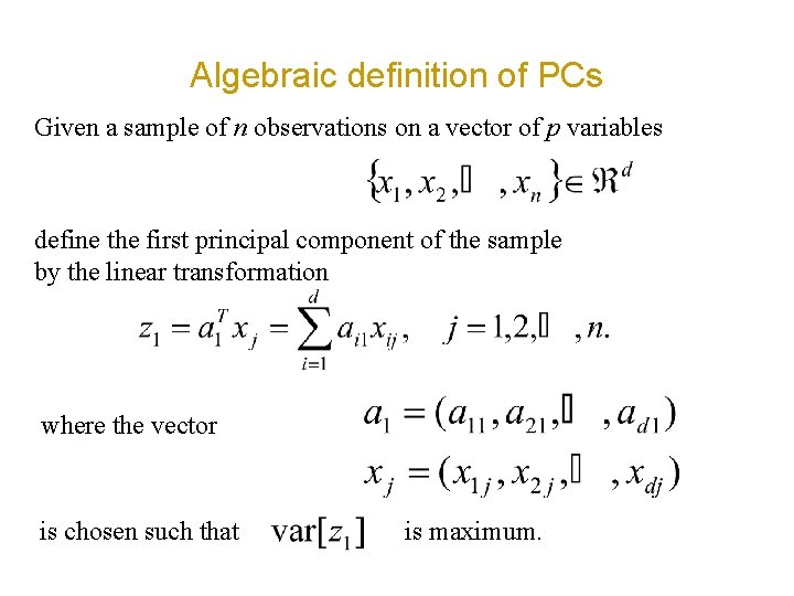
Algebraic definition of PCs Given a sample of n observations on a vector of p variables define the first principal component of the sample by the linear transformation where the vector is chosen such that is maximum.

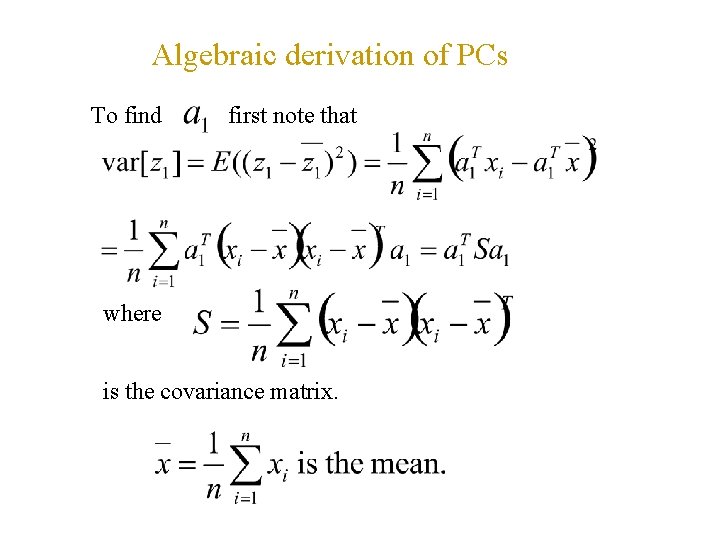
Algebraic derivation of PCs To find first note that where is the covariance matrix.

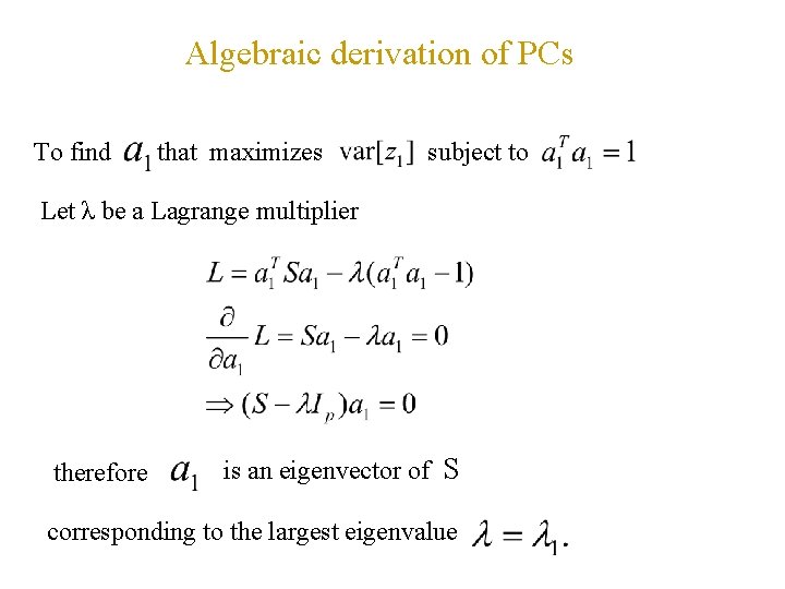
Algebraic derivation of PCs To find that maximizes subject to Let λ be a Lagrange multiplier therefore is an eigenvector of S corresponding to the largest eigenvalue

Algebraic derivation of PCs We find that whose eigenvalue is also an eigenvector of S is the second largest. In general • The kth largest eigenvalue of S is the variance of the kth PC. • The kth PC retains the kth greatest fraction of the variation in the sample.

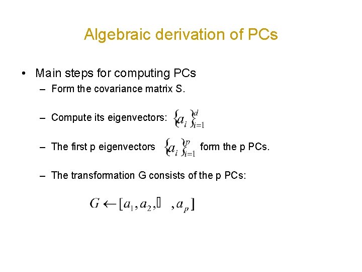
Algebraic derivation of PCs • Main steps for computing PCs – Form the covariance matrix S. – Compute its eigenvectors: – The first p eigenvectors form the p PCs. – The transformation G consists of the p PCs:

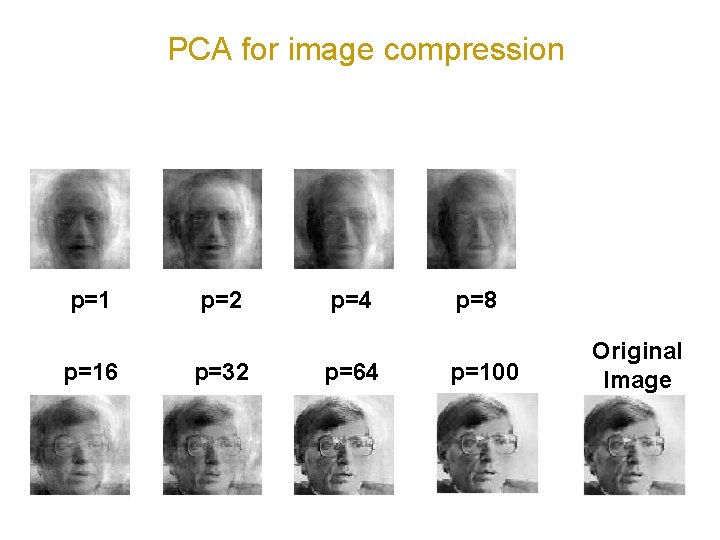
PCA for image compression p=16 p=2 p=32 p=4 p=64 p=8 p=100 Original Image

Outline of lecture • What is feature reduction? • Why feature reduction? • Feature reduction algorithms – Principal Component Analysis (PCA) – Linear Discriminant Analysis (LDA)

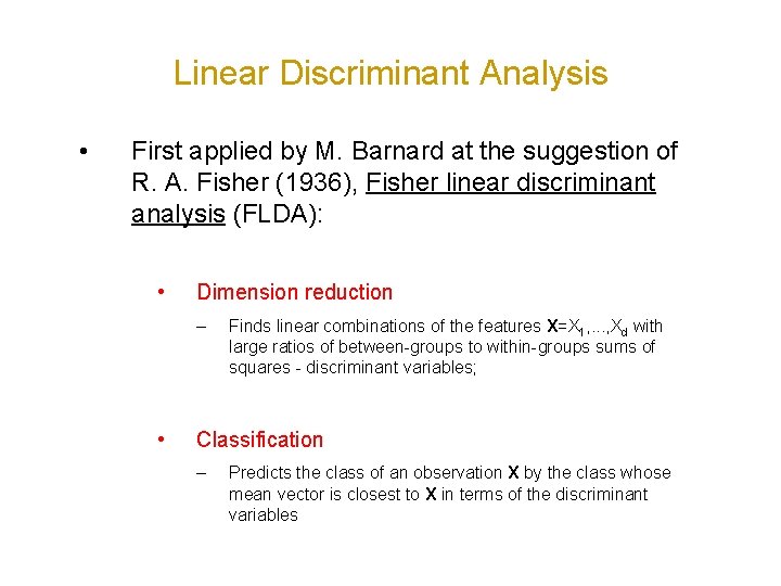
Linear Discriminant Analysis • First applied by M. Barnard at the suggestion of R. A. Fisher (1936), Fisher linear discriminant analysis (FLDA): • Dimension reduction – • Finds linear combinations of the features X=X 1, . . . , Xd with large ratios of between-groups to within-groups sums of squares - discriminant variables; Classification – Predicts the class of an observation X by the class whose mean vector is closest to X in terms of the discriminant variables

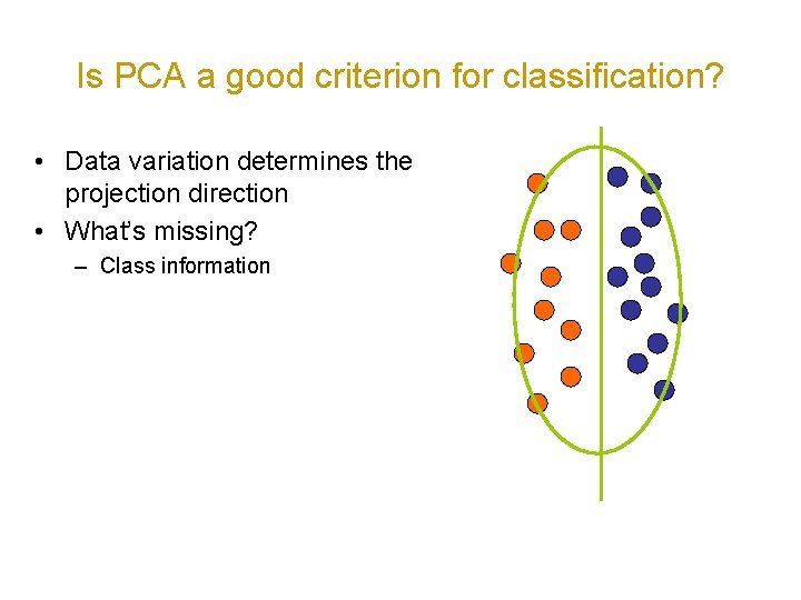
Is PCA a good criterion for classification? • Data variation determines the projection direction • What’s missing? – Class information

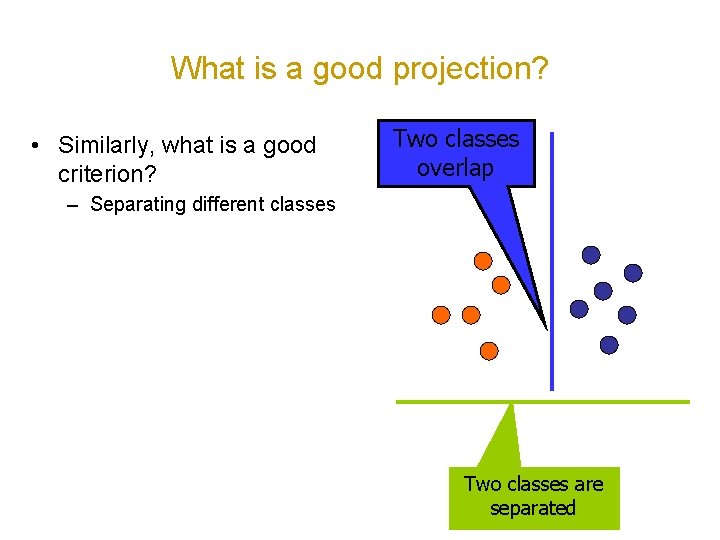
What is a good projection? • Similarly, what is a good criterion? Two classes overlap – Separating different classes Two classes are separated

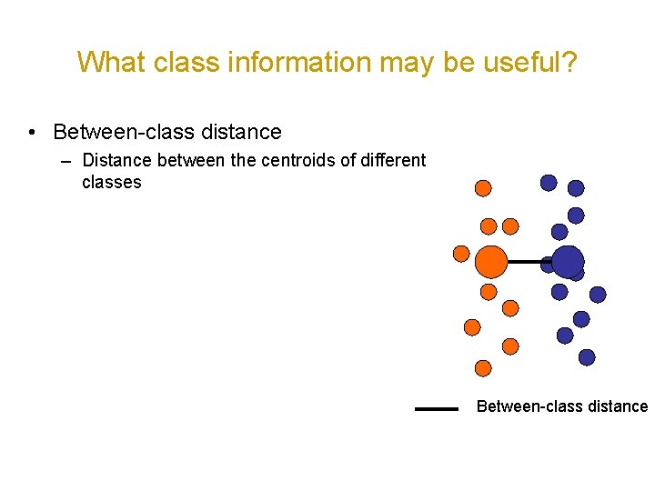
What class information may be useful? • Between-class distance – Distance between the centroids of different classes Between-class distance

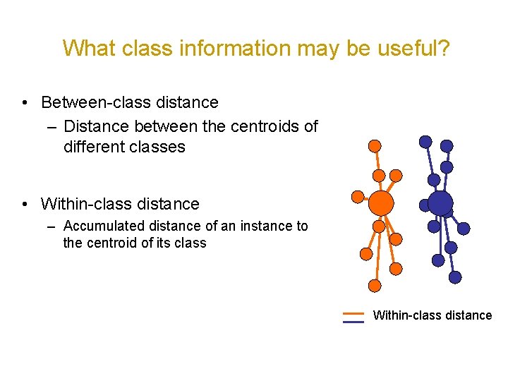
What class information may be useful? • Between-class distance – Distance between the centroids of different classes • Within-class distance – Accumulated distance of an instance to the centroid of its class Within-class distance

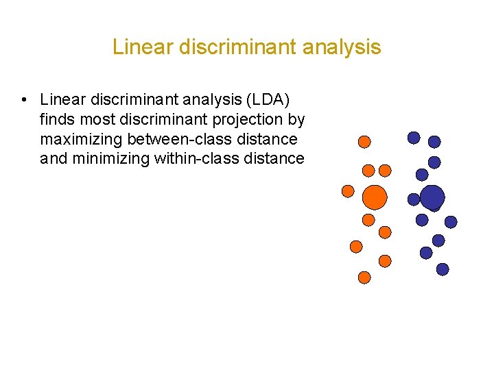
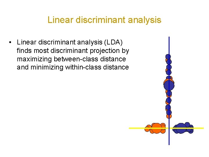
Linear discriminant analysis • Linear discriminant analysis (LDA) finds most discriminant projection by maximizing between-class distance and minimizing within-class distance

Linear discriminant analysis • Linear discriminant analysis (LDA) finds most discriminant projection by maximizing between-class distance and minimizing within-class distance

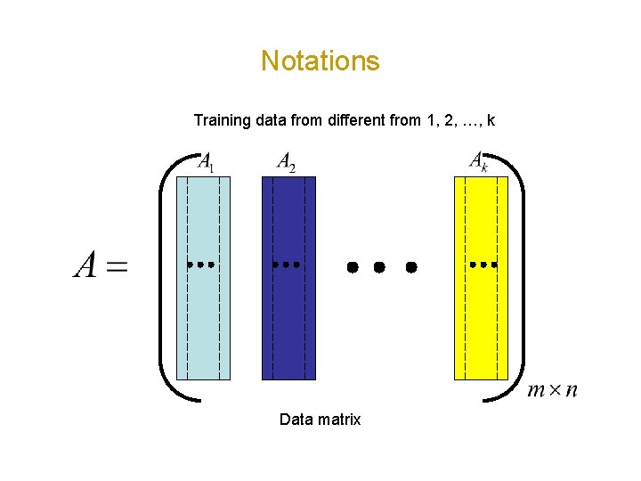
Notations Training data from different from 1, 2, …, k Data matrix

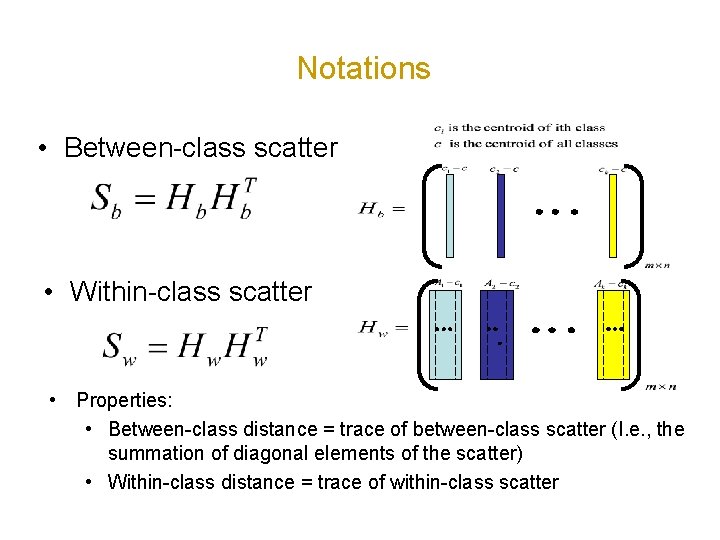
Notations • Between-class scatter • Within-class scatter • Properties: • Between-class distance = trace of between-class scatter (I. e. , the summation of diagonal elements of the scatter) • Within-class distance = trace of within-class scatter

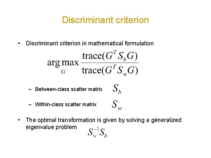
Discriminant criterion • Discriminant criterion in mathematical formulation – Between-class scatter matrix – Within-class scatter matrix • The optimal transformation is given by solving a generalized eigenvalue problem

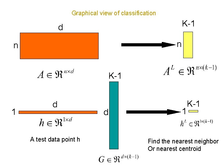
Graphical view of classification K-1 d n n K-1 1 d A test data point h d 1 K-1 Find the nearest neighbor Or nearest centroid

Applications • Face recognition – Belhumeour et al. , PAMI’ 97 • Image retrieval – Swets and Weng, PAMI’ 96 • Gene expression data analysis – Dudoit et al. , JASA’ 02; Ye et al. , TCBB’ 04 • Protein expression data analysis • Lilien et al. , Comp. Bio. ’ 03 • Text mining – Park et al. , SIMAX’ 03; Ye et al. , PAMI’ 04 • Medical image analysis – Dundar, SDM’ 05