Preprocessing Exploration Feature selection Dimensionality reduction feature extraction

Σκοποί ενότητας Εισαγωγή και εξοικείωση με τις μεθόδους Preprocessing, Exploration, Feature selection, Dimensionality reduction, feature extraction and evaluation. 4

Περιεχόμενα ενότητας • Pre-processing • Exploration • Feature selection • Dimensionality reduction • Feature extraction and evaluation 5

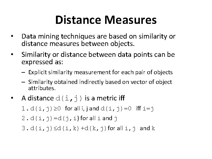
Distance Measures • • Data mining techniques are based on similarity or distance measures between objects. Similarity or distance between data points can be expressed as: – Explicit similarity measurement for each pair of objects – Similarity obtained indirectly based on vector of object attributes. • A distance d(i, j) is a metric iff 1. d(i, j) 0 for all i, j and d(i, j)=0 iff i=j 2. d(i, j)=d(j, i) for all i and j 3. d(i, j) d(i, k)+d(k, j)for all i, j and k

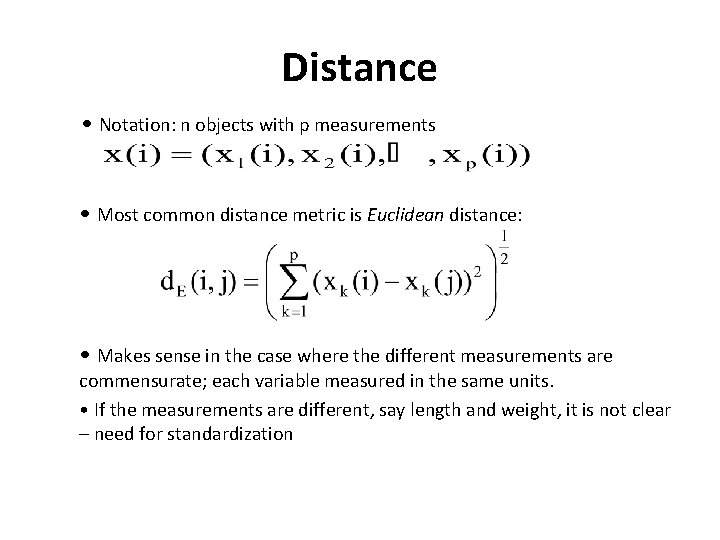
Distance • Notation: n objects with p measurements • Most common distance metric is Euclidean distance: • Makes sense in the case where the different measurements are commensurate; each variable measured in the same units. • If the measurements are different, say length and weight, it is not clear – need for standardization

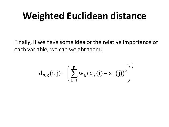
Weighted Euclidean distance Finally, if we have some idea of the relative importance of each variable, we can weight them:

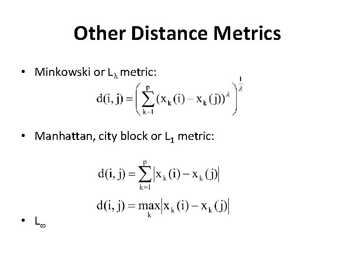
Other Distance Metrics • Minkowski or L metric: • Manhattan, city block or L 1 metric: • L

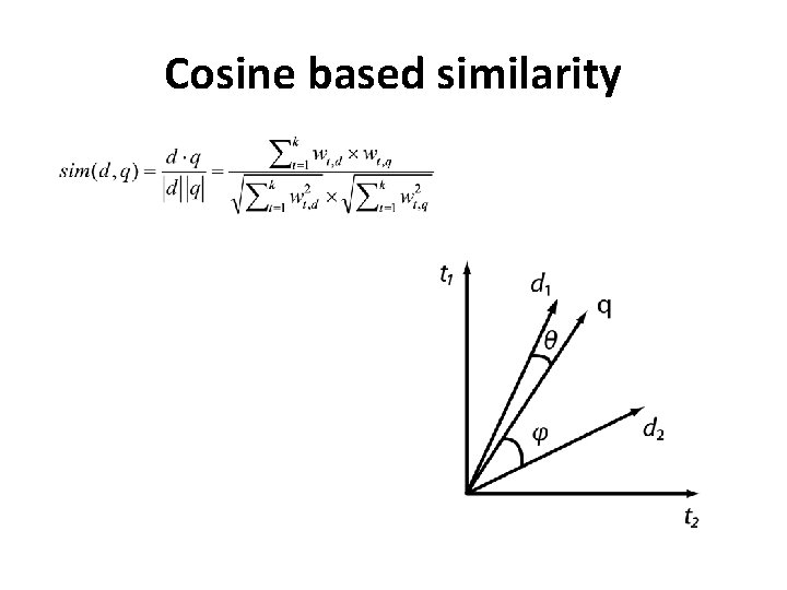
Cosine based similarity

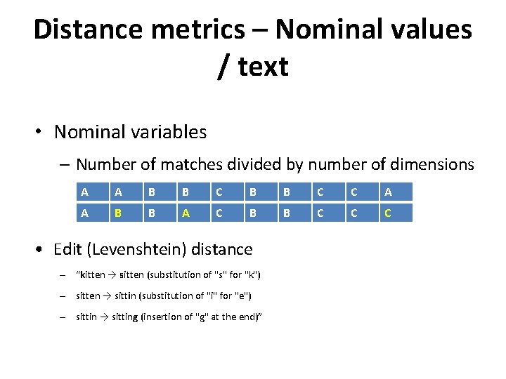
Distance metrics – Nominal values / text • Nominal variables – Number of matches divided by number of dimensions A A B B C C A A B B A C B B C C C • Edit (Levenshtein) distance – “kitten → sitten (substitution of "s" for "k") – sitten → sittin (substitution of "i" for "e") – sittin → sitting (insertion of "g" at the end)”

Exploratory Data Analysis • Methods not including formal statistical modeling and inference – Detection of mistakes – Checking of assumptions – Preliminary selection of appropriate models – Determining relationships among the explanatory variables, and – Assessing the direction and rough size of relationships between explanatory and outcome variables (i. e. demographics – purchase) • Useful information about the data – Min and Max values – Mean Value – Standard Deviation – Number of instances per value (for nominal data) – Percentage of missing values – Data distribution

Data Quality • Individual measurements – Random noise in individual measurements • Variance (precision) • Bias • Random data entry errors • Noise in label assignment (e. g. , class labels in medical data sets) – Systematic errors • E. g. , all ages > 99 recorded as 99 • More individuals aged 20, 30, 40, etc than expected – Missing information • Missing at random – • Questions on a questionnaire that people randomly forget to fill in Missing systematically – Questions that people don’t want to answer – Patients who are too ill for a certain test

Data Quality – Ideal case = random sample from population of interest – Real case = often a biased sample of some sort – Key point: patterns or models from training data are valid on future (test) data only if they are generated from the same probability distribution • Examples of non-randomly sampled data – Medical study where subjects are all students – Geographic dependencies – Temporal dependencies – Stratified samples • E. g. , 50% healthy, 50% ill – Hidden systematic effects • E. g. , market basket data the weekend of a large sale in the store • E. g. , Web log data during finals week

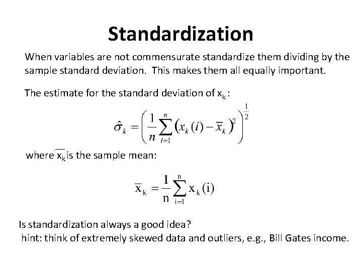
Standardization When variables are not commensurate standardize them dividing by the sample standard deviation. This makes them all equally important. The estimate for the standard deviation of xk : where xk is the sample mean: Is standardization always a good idea? hint: think of extremely skewed data and outliers, e. g. , Bill Gates income.

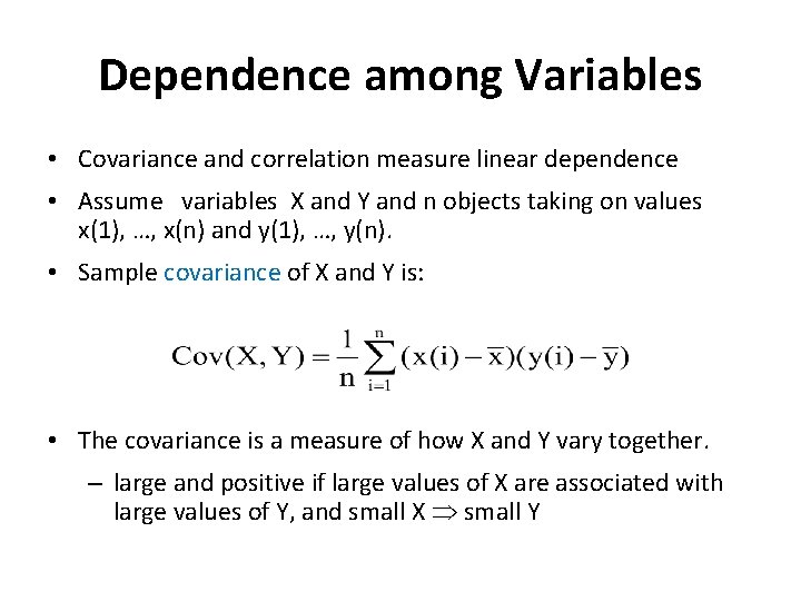
Dependence among Variables • Covariance and correlation measure linear dependence • Assume variables X and Y and n objects taking on values x(1), …, x(n) and y(1), …, y(n). • Sample covariance of X and Y is: • The covariance is a measure of how X and Y vary together. – large and positive if large values of X are associated with large values of Y, and small X small Y

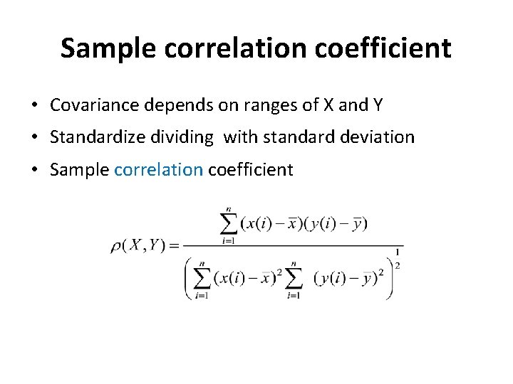
Sample correlation coefficient • Covariance depends on ranges of X and Y • Standardize dividing with standard deviation • Sample correlation coefficient

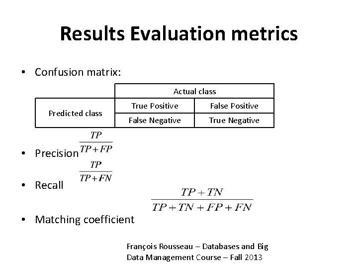
Results Evaluation metrics • Confusion matrix: Actual class Predicted class True Positive False Negative True Negative • Precision • Recall • Matching coefficient François Rousseau – Databases and Big Data Management Course – Fall 2013

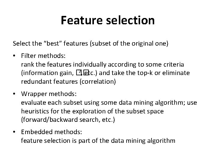
Feature selection Select the “best” features (subset of the original one) • Filter methods: rank the features individually according to some criteria 2, etc. ) and take the top-k or eliminate (information gain, �� redundant features (correlation) • Wrapper methods: evaluate each subset using some data mining algorithm; use heuristics for the exploration of the subset space (forward/backward search, etc. ) • Embedded methods: feature selection is part of the data mining algorithm

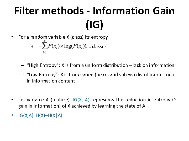
Filter methods - Information Gain (IG) • For a random variable X (class) its entropy H= , c classes – “High Entropy”: X is from a uniform distribution – lack on information – “Low Entropy”: X is from varied (peaks and valleys) distribution – rich in information content • Let variable A (feature), IG(X, A) represents the reduction in entropy (~ gain in Information) of X achieved by learning the state of A: • IG(X, A)=H(X)–H(X|A)

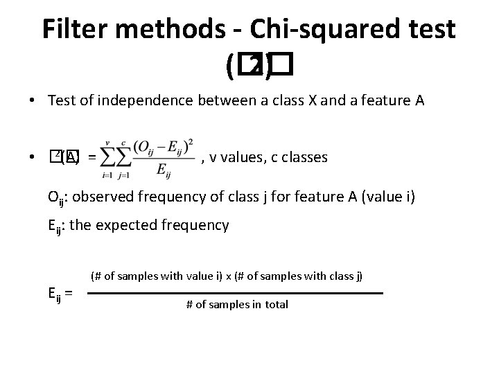
Filter methods - Chi-squared test (�� 2) • Test of independence between a class X and a feature A 2(A) = • �� , v values, c classes Oij: observed frequency of class j for feature A (value i) Eij: the expected frequency Eij = (# of samples with value i) x (# of samples with class j) # of samples in total

Finding the k best variables • Find the subset of k variables that predicts best: – This is a generic problem when p is large (arises with all types of models, not just linear regression) • Models with different complexity. . • p models with a single variable • p(p-1)/2 models with 2 variables, etc • … • 2 p possible models in total • Best k set is not the same as the best k individual variables • What does “best” mean here?

Search Problem • How can we search over all 2 p possible models? – exhaustive search is clearly infeasible • Heuristic search is used to search over model space: • Forward search (greedy) • Backward search (greedy) • Branch and bound techniques • Variable selection problem in several data mining algorithms • Outer loop that searches over variable combinations • Inner loop that evaluates each combination

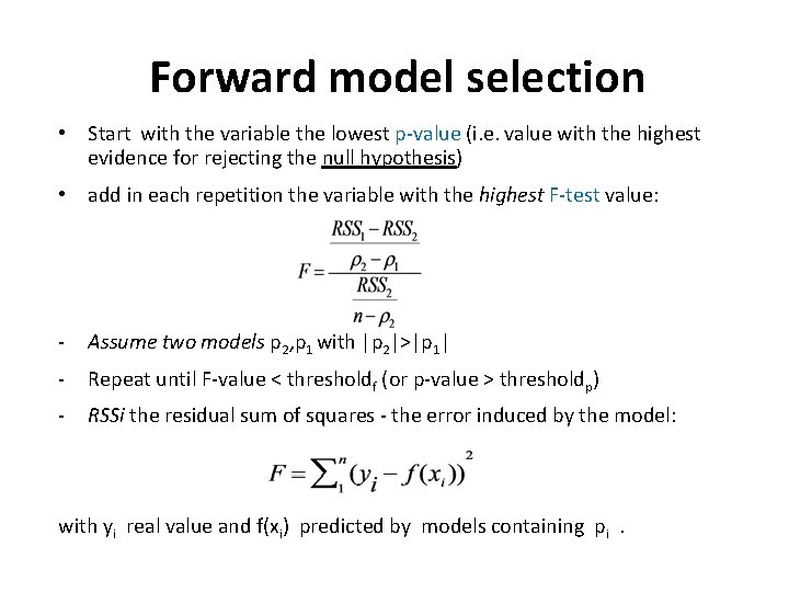
Forward model selection • Start with the variable the lowest p-value (i. e. value with the highest evidence for rejecting the null hypothesis) • add in each repetition the variable with the highest F-test value: - Assume two models p 2, p 1 with |p 2|>|p 1| - Repeat until F-value < thresholdf (or p-value > thresholdp) - RSSi the residual sum of squares - the error induced by the model: with yi real value and f(xi) predicted by models containing pi.

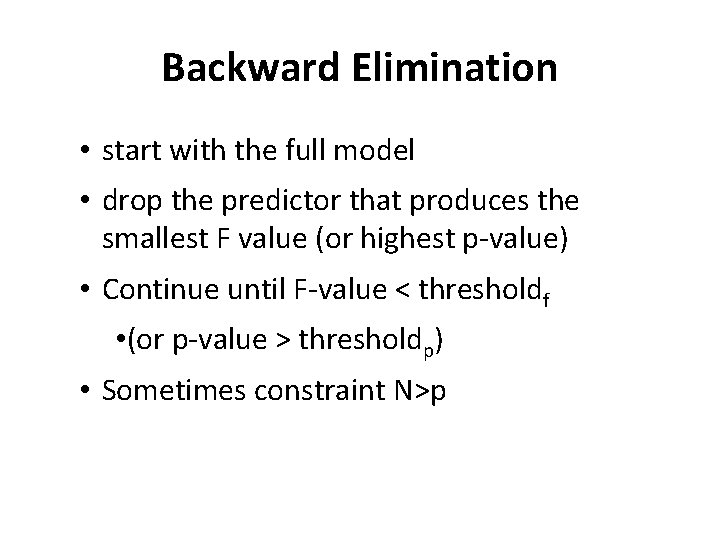
Backward Elimination • start with the full model • drop the predictor that produces the smallest F value (or highest p-value) • Continue until F-value < thresholdf • (or p-value > thresholdp) • Sometimes constraint N>p

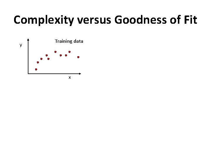
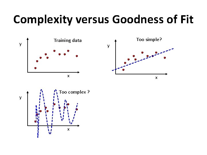
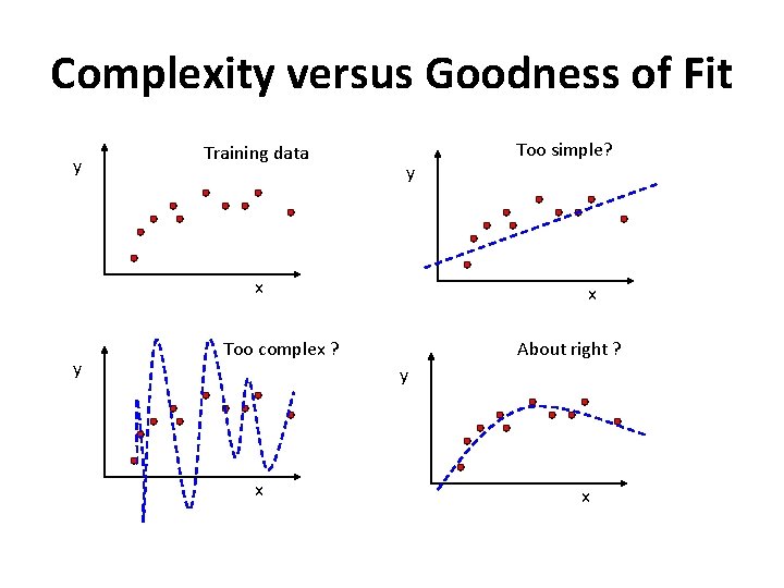
Complexity versus Goodness of Fit y Training data x

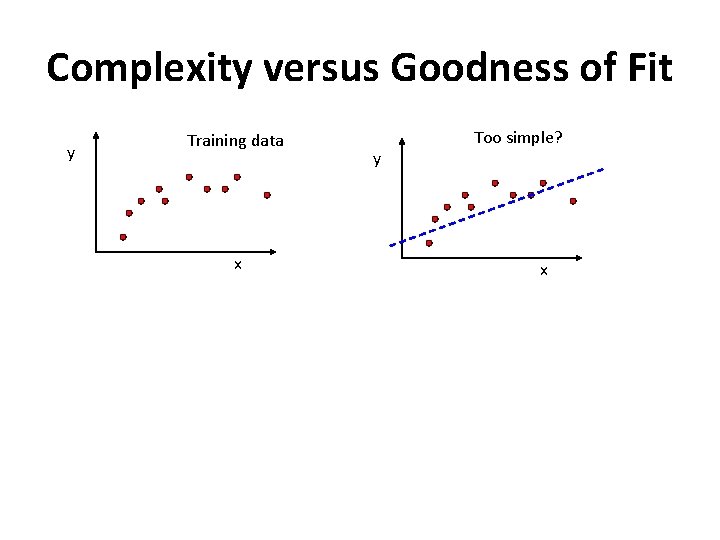
Complexity versus Goodness of Fit y Training data x y Too simple? x

Complexity versus Goodness of Fit y Training data x y Too complex ? x y Too simple? x

Complexity versus Goodness of Fit y Training data y x y Too simple? x Too complex ? About right ? y x x

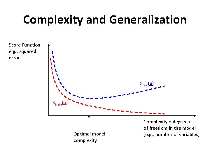
Complexity and Generalization Score Function e. g. , squared error Stest(q) Strain(q) Optimal model complexity Complexity = degrees of freedom in the model (e. g. , number of variables)

Useful References • Principles of Data Mining, David J. Hand, Heikki Mannila and Padhraic Smyth MIT Press 2001 • T. Hastie, R. Tibshirani, and J. Friedman, Elements of Statistical Learning, Springer Verlag, 2001 • Dash, Manoranjan, and Huan Liu. "Feature selection for classification. “ Intelligent data analysis 1. 1 -4 (1997): 131 -156. • N. R. Draper and H. Smith, Applied Regression Analysis, 2 nd edition, Wiley, 1981 (the “bible” for classical regression methods in statistics • An introduction to variable and feature selection, Isabelle Guyon, André Elisseeff, The Journal of Machine Learning Researchive Volume 3, 3/1/2003, pp. 1157 -1182 • Mohammed J. Zaki, course notes, High Dimesional Notes http: //www. cs. rpi. edu/~zaki/wwwnew/uploads/Dmcourse/Main/chap 6. pdf

Data features • Huge volume/ Dimensionality • Heterogeneity • Dynamism – Motion – Availability? – Frequent Updates • Huge query loads • Examples: Web, P 2 P systems, Image data

Curse of Dimensionality • Some coordinates do not contribute to the data representation. • Subsets of the dimensions may be highly correlated. • Nearest neighbor is distorted in a high dimensional space Low dimension intuitions do not apply to high dimensions • Empty space phenomenon

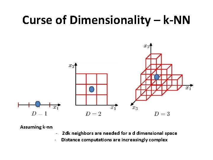
Curse of Dimensionality – k-NN Assuming k-nn - 2 dk neighbors are needed for a d dimensional space - Distance computations are increasingly complex

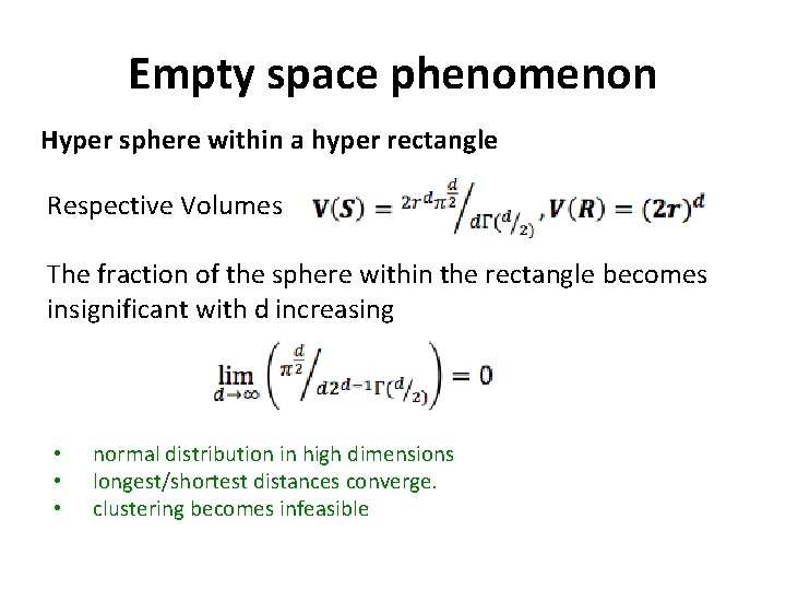
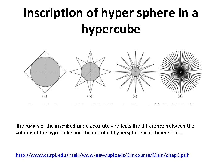
Empty space phenomenon Hyper sphere within a hyper rectangle Respective Volumes The fraction of the sphere within the rectangle becomes insignificant with d increasing • • • normal distribution in high dimensions longest/shortest distances converge. clustering becomes infeasible

Inscription of hyper sphere in a hypercube The radius of the inscribed circle accurately reflects the difference between the volume of the hypercube and the inscribed hypersphere in d-dimensions. http: //www. cs. rpi. edu/~zaki/www-new/uploads/Dmcourse/Main/chap 6. pdf

Dim. Reduction – Linear Algorithms • • • Matrix Factorization methods Principal Components Analysis (PCA) Singular Value Decomposition (SVD) Multidimensional Scaling (MDS) Non negative Matrix Factorization (NMF) Latent Semantic Indexing (LSI)

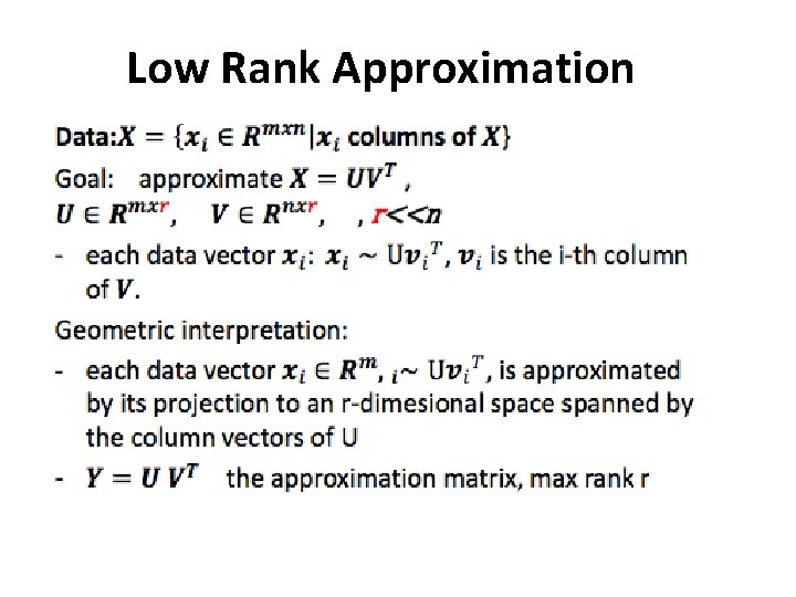
Low Rank Approximation

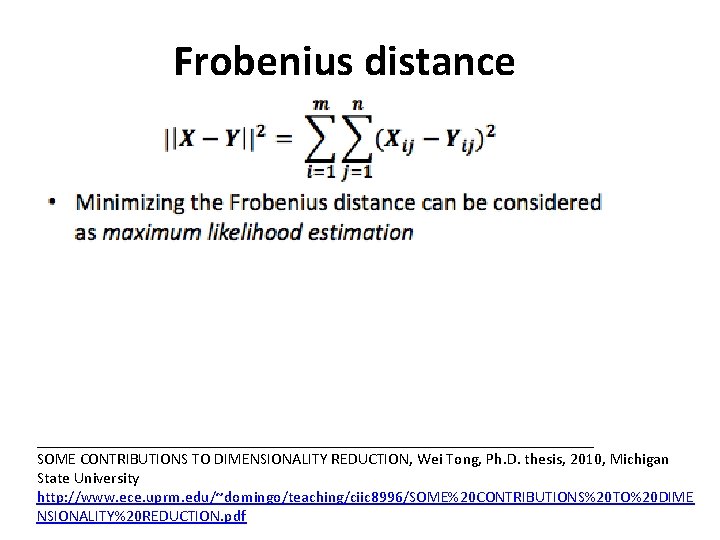
Frobenius distance ___________________________________ SOME CONTRIBUTIONS TO DIMENSIONALITY REDUCTION, Wei Tong, Ph. D. thesis, 2010, Michigan State University http: //www. ece. uprm. edu/~domingo/teaching/ciic 8996/SOME%20 CONTRIBUTIONS%20 TO%20 DIME NSIONALITY%20 REDUCTION. pdf

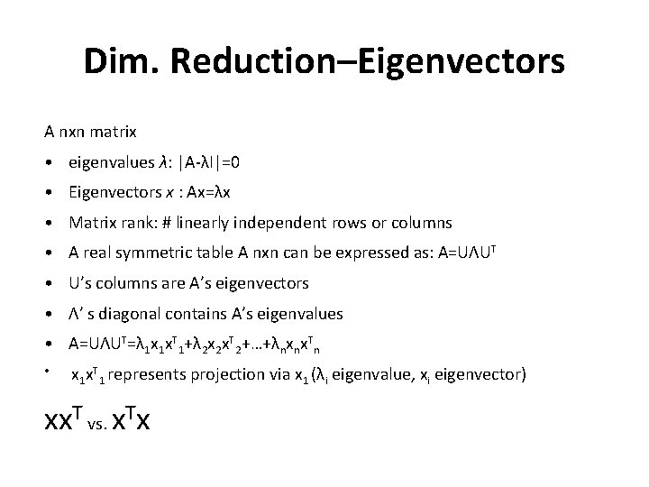
Dim. Reduction–Eigenvectors A nxn matrix • eigenvalues λ: |Α-λΙ|=0 • Eigenvectors x : Ax=λx • Matrix rank: # linearly independent rows or columns • A real symmetric table Α nxn can be expressed as: A=UΛUT • U’s columns are Α’s eigenvectors • Λ’ s diagonal contains Α’s eigenvalues • Α=UΛUT=λ 1 x 1 x. T 1+λ 2 x 2 x. T 2+…+λnxnx. Tn • x 1 x. T 1 represents projection via x 1 (λi eigenvalue, xi eigenvector) xx. T vs. x. Tx

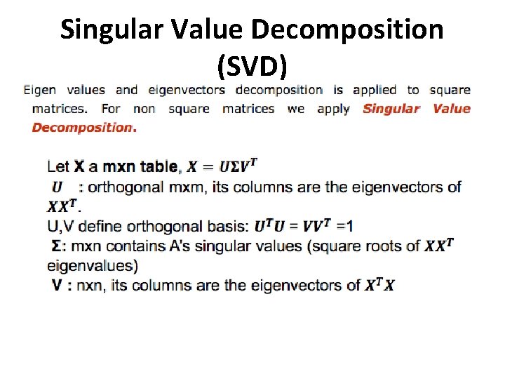
Singular Value Decomposition (SVD)

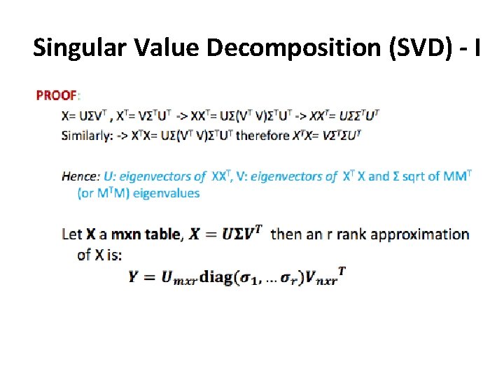
Singular Value Decomposition (SVD) - I

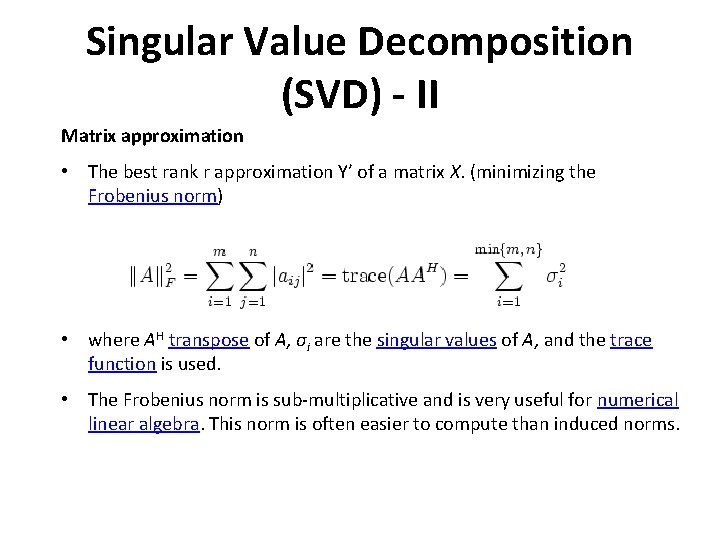
Singular Value Decomposition (SVD) - II Matrix approximation • The best rank r approximation Y’ of a matrix X. (minimizing the Frobenius norm) • where AH transpose of A, σi are the singular values of A, and the trace function is used. • The Frobenius norm is sub-multiplicative and is very useful for numerical linear algebra. This norm is often easier to compute than induced norms.

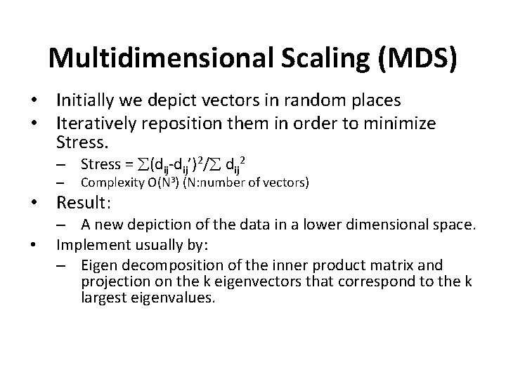
Multidimensional Scaling (MDS) • Initially we depict vectors in random places • Iteratively reposition them in order to minimize Stress. – Stress = (dij-dij’)2/ dij 2 – Complexity Ο(N 3) (Ν: number of vectors) • Result: • – A new depiction of the data in a lower dimensional space. Implement usually by: – Eigen decomposition of the inner product matrix and projection on the k eigenvectors that correspond to the k largest eigenvalues.

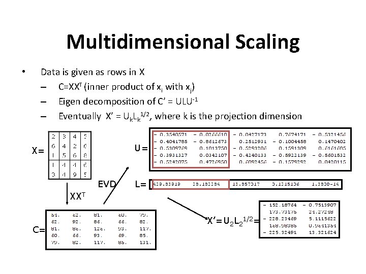
Multidimensional Scaling • Data is given as rows in Χ – C=XXT (inner product of xi with xj) – Eigen decomposition of C’ = ULU-1 – Eventually X’ = Uk. Lk 1/2, where k is the projection dimension U= X= EVD L= XXT C= L= X’=U 2 L 21/2=

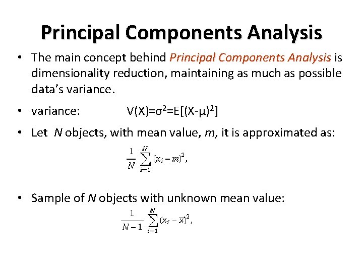
Principal Components Analysis • The main concept behind Principal Components Analysis is dimensionality reduction, maintaining as much as possible data’s variance. • variance: V(X)=σ2=Ε[(Χ-μ)2] • Let Ν objects, with mean value, m, it is approximated as: • Sample of Ν objects with unknown mean value:

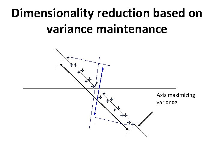
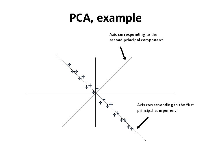
Dimensionality reduction based on variance maintenance Axis maximizing variance

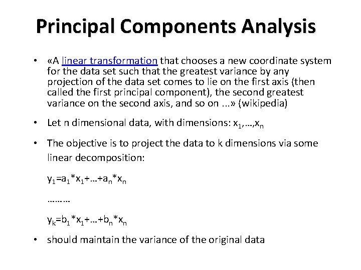
Principal Components Analysis • «Α linear transformation that chooses a new coordinate system for the data set such that the greatest variance by any projection of the data set comes to lie on the first axis (then called the first principal component), the second greatest variance on the second axis, and so on. . . » (wikipedia) • Let n dimensional data, with dimensions: x 1, …, xn • The objective is to project the data to k dimensions via some linear decomposition: y 1=a 1*x 1+…+an*xn ……… yk=b 1*x 1+…+bn*xn • should maintain the variance of the original data

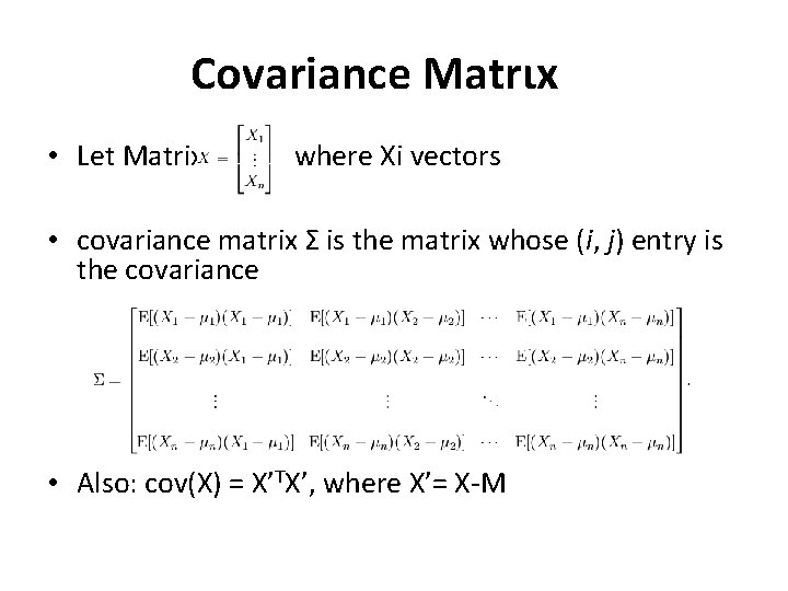
Covariance Μatrιx • Let Matrix where Xi vectors • covariance matrix Σ is the matrix whose (i, j) entry is the covariance • Also: cov(X) = X’TX’, where X’= X-M

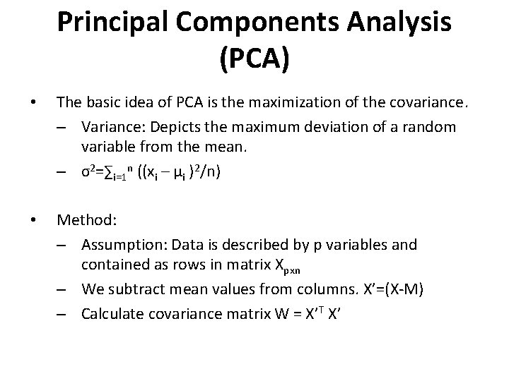
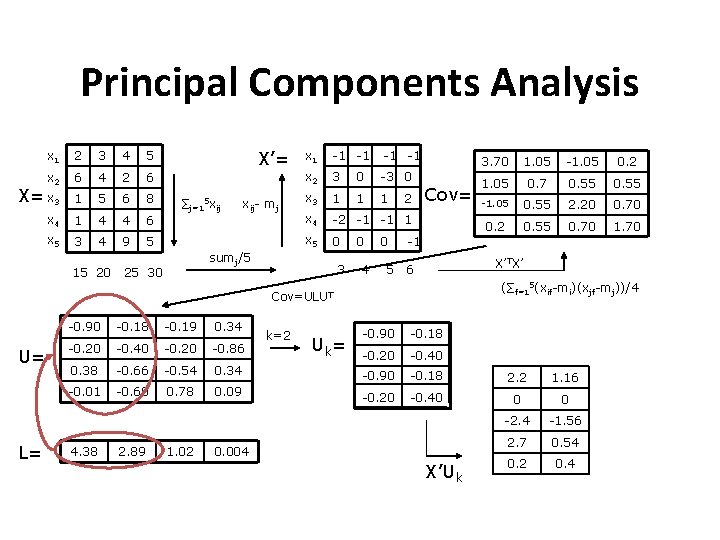
Principal Components Analysis (PCA) • The basic idea of PCA is the maximization of the covariance. – Variance: Depicts the maximum deviation of a random variable from the mean. – σ2=∑i=1 n ((xi – μi )2/n) • Method: – Assumption: Data is described by p variables and contained as rows in matrix Xpxn – We subtract mean values from columns. X’=(X-M) – Calculate covariance matrix W = X’T X’

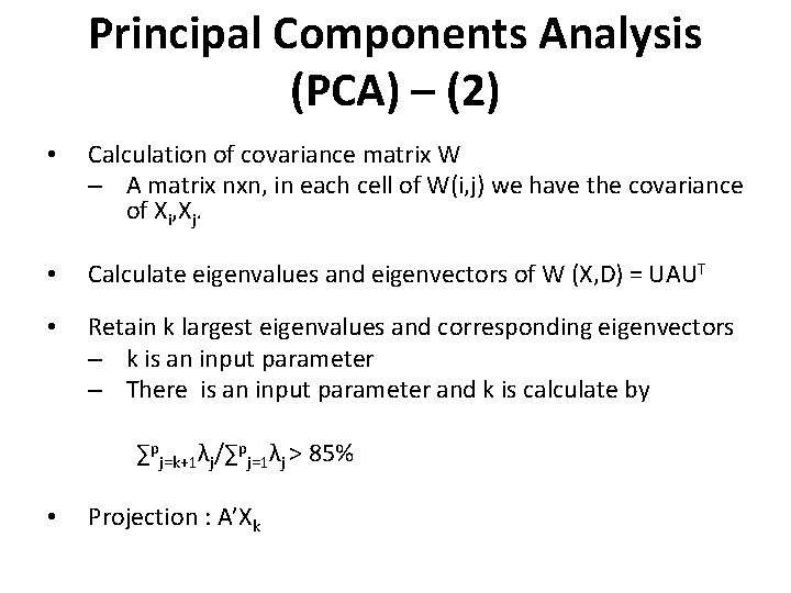
Principal Components Analysis (PCA) – (2) • Calculation of covariance matrix W – A matrix nxn, in each cell of W(i, j) we have the covariance of Xi, Xj. • Calculate eigenvalues and eigenvectors of W (X, D) = UAUT • Retain k largest eigenvalues and corresponding eigenvectors – k is an input parameter – There is an input parameter and k is calculate by ∑pj=k+1λj/∑pj=1λj > 85% • Projection : A’Χk

Principal Components Analysis -1 -1 x 2 3 0 -3 0 x 3 1 1 1 6 x 4 -2 -1 -1 1 5 x 5 0 2 3 4 5 x 2 6 4 2 6 1 5 6 8 X= x 3 x 4 x 5 1 3 4 4 15 20 4 9 X’= x 1 ∑j=15 xij xij- mj sumj/5 25 30 3 0 4 0 5 2 Cov= U= L= -0. 18 -0. 19 0. 34 -0. 20 -0. 40 -0. 20 -0. 86 0. 38 -0. 66 -0. 54 0. 34 -0. 01 -0. 60 0. 78 0. 09 4. 38 2. 89 1. 02 k=2 Uk= 1. 05 -1. 05 0. 2 1. 05 0. 7 0. 55 -1. 05 0. 55 2. 20 0. 70 0. 2 0. 55 0. 70 1. 70 -1 X’TX’ 6 (∑f=15(xif-mi)(xjf-mj))/4 Cov=ULUT -0. 90 3. 70 -0. 90 -0. 18 -0. 20 -0. 40 -0. 90 -0. 18 2. 2 1. 16 -0. 20 -0. 40 0 0 -2. 4 -1. 56 2. 7 0. 54 0. 2 0. 4 0. 004 X’Uk

PCA, example Axis corresponding to the second principal component Axis corresponding to the first principal component

PCA Synopsis & Applications - Preprocessing step preceding the application of data mining algorithms (such as clustering). - Data Visualization & Noise reduction. • - It is a dimensionality reduction method • - Nominal complexity Ο( np^2+p^3) – n: number of data points – p: number of initial space dimensions • - The new space maintains sufficiently the data variance.

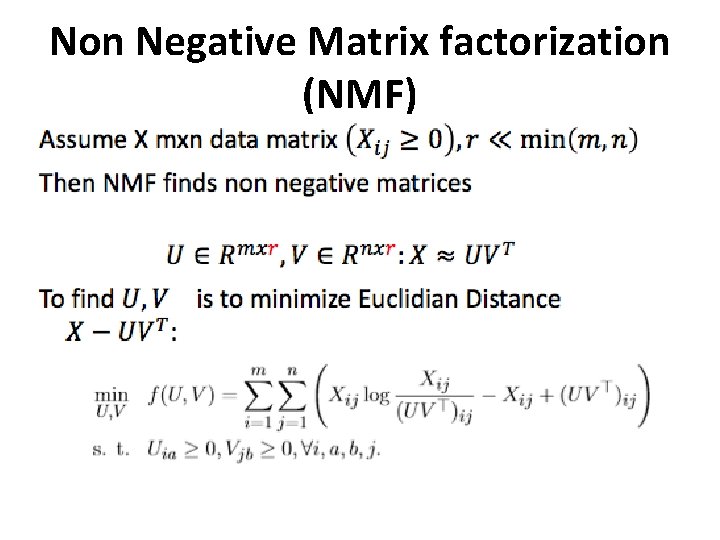
Non Negative Matrix factorization (NMF) • - Applying SVD results in factorized matrices with positive and negative elements may contradict the physical meaning of the result. • Example: • - X gray-scale image intensities, Y its SVD approximation • - difficult to interpret the reconstructed matrix Y for a gray-scale image with negative elements. • - Nonnegative matrix factorization (NMF) • find the reduced rank nonnegative factors to approximate a given nonnegative data matrix.

Non Negative Matrix factorization (NMF)

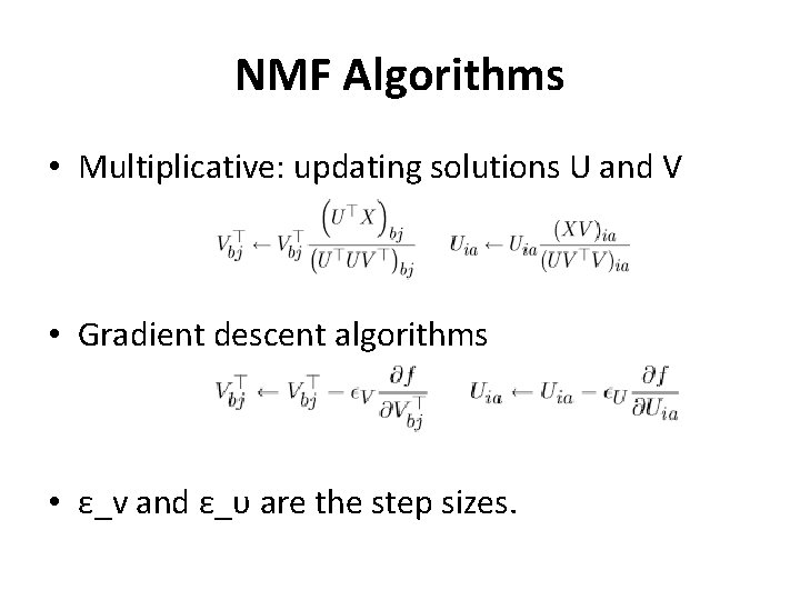
NMF Algorithms • Multiplicative: updating solutions U and V • Gradient descent algorithms • ε_v and ε_υ are the step sizes.

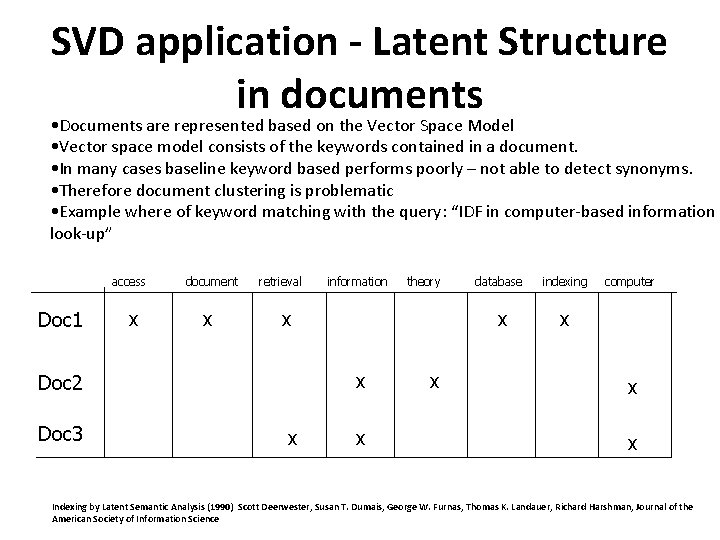
SVD application - Latent Structure in documents • Documents are represented based on the Vector Space Model • Vector space model consists of the keywords contained in a document. • In many cases baseline keyword based performs poorly – not able to detect synonyms. • Therefore document clustering is problematic • Example where of keyword matching with the query: “IDF in computer-based information look-up” access Doc 1 x document x retrieval theory x x database x x Doc 2 Doc 3 information x x indexing computer x x x Indexing by Latent Semantic Analysis (1990) Scott Deerwester, Susan T. Dumais, George W. Furnas, Thomas K. Landauer, Richard Harshman, Journal of the American Society of Information Science

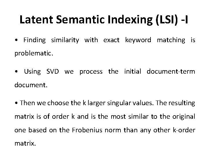
Latent Semantic Indexing (LSI) -I • Finding similarity with exact keyword matching is problematic. • Using SVD we process the initial document-term document. • Then we choose the k larger singular values. The resulting matrix is of order k and is the most similar to the original one based on the Frobenius norm than any other k-order matrix.

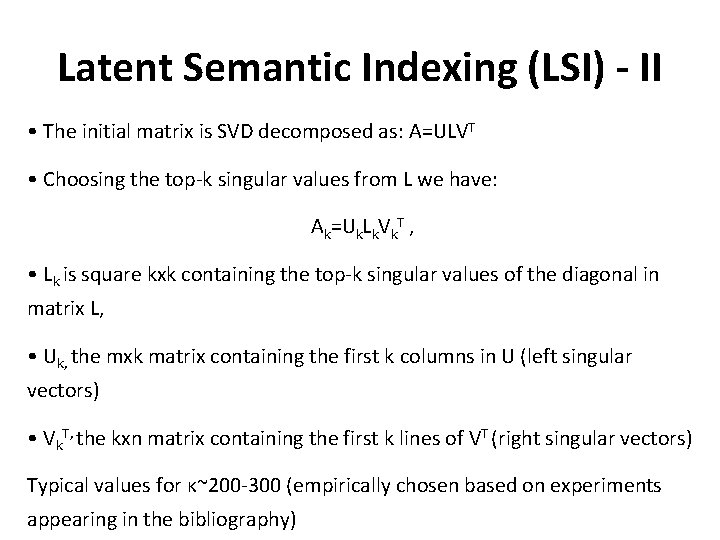
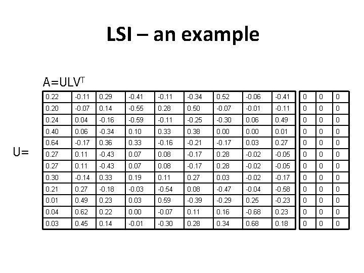
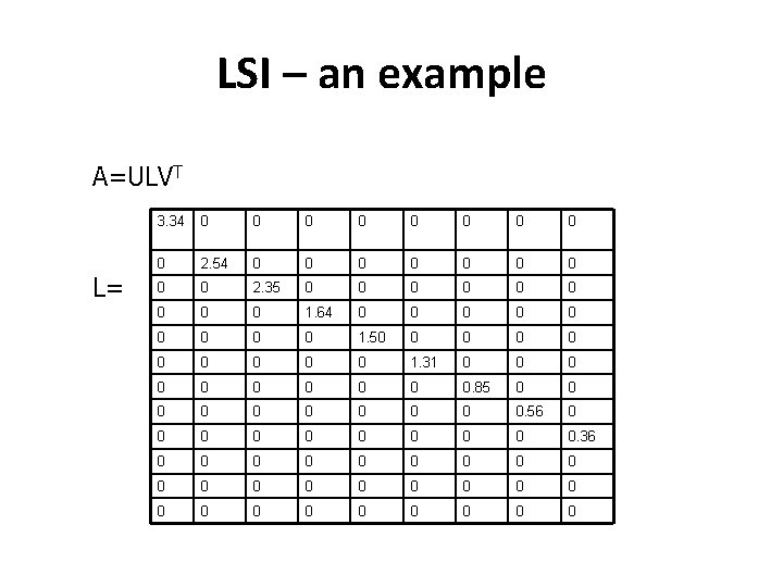
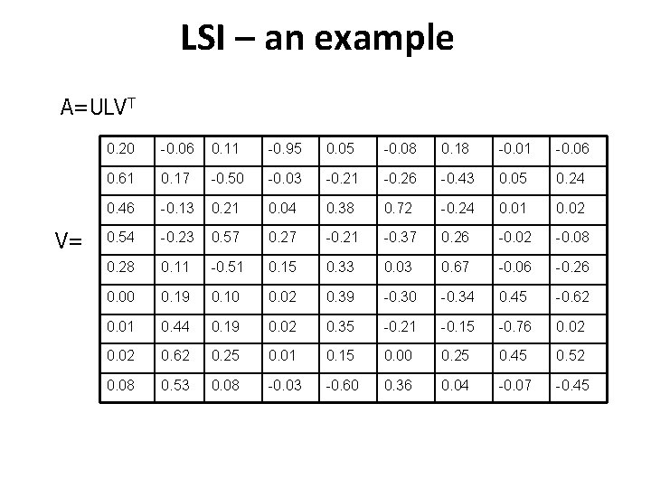
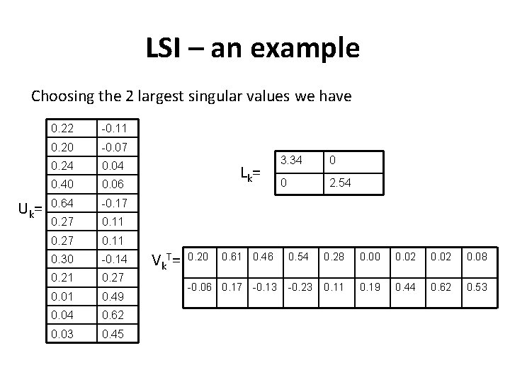
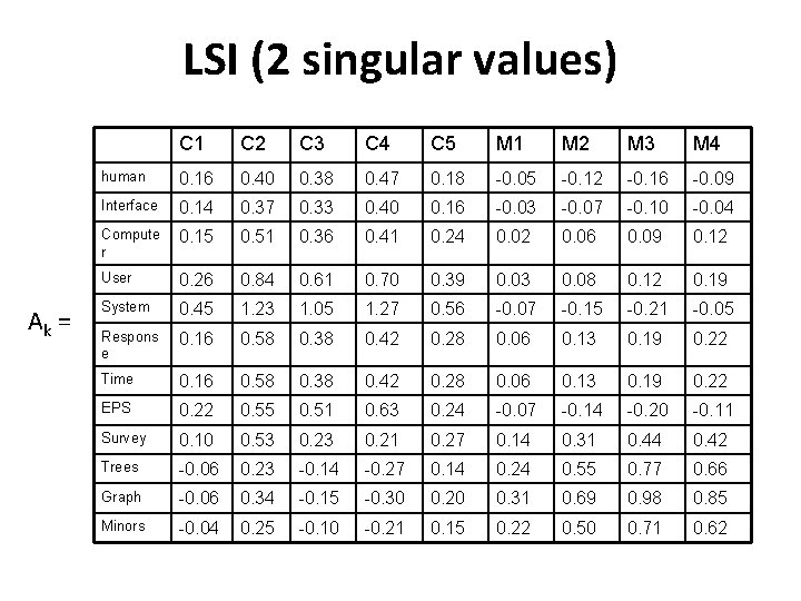
Latent Semantic Indexing (LSI) - II • The initial matrix is SVD decomposed as: Α=ULVT • Choosing the top-k singular values from L we have: Αk=Uk. Lk. Vk. T , • Lk is square kxk containing the top-k singular values of the diagonal in matrix L, • Uk, the mxk matrix containing the first k columns in U (left singular vectors) • Vk. T, the kxn matrix containing the first k lines of VT (right singular vectors) Typical values for κ~200 -300 (empirically chosen based on experiments appearing in the bibliography)

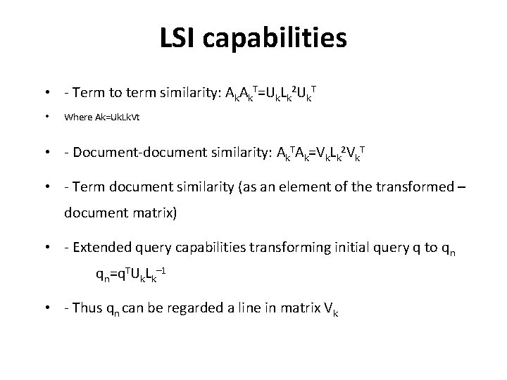
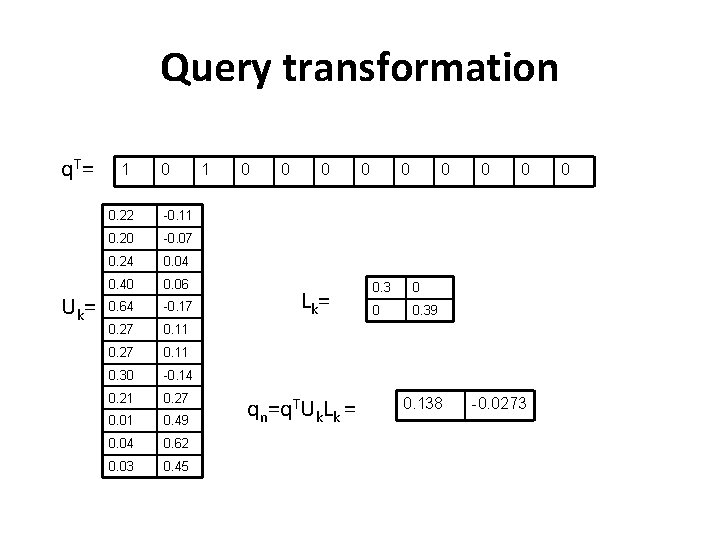
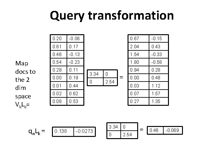
LSI capabilities • - Term to term similarity: ΑkΑk. T=Uk. Lk 2 Uk. T • Where Ak=Uk. Lk. Vt • - Document-document similarity: Αk. TΑk=Vk. Lk 2 Vk. T • - Term document similarity (as an element of the transformed – document matrix) • - Extended query capabilities transforming initial query q to qn qn=q. TUk. Lk– 1 • - Thus qn can be regarded a line in matrix Vk

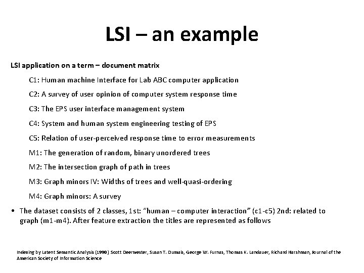
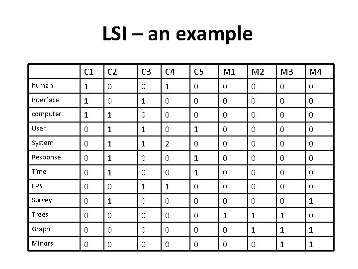
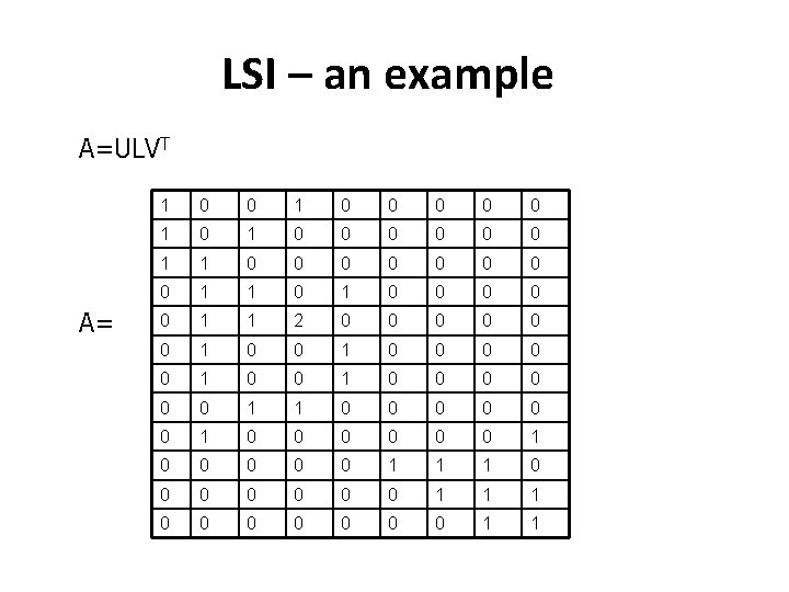
LSI – an example LSI application on a term – document matrix C 1: Human machine Interface for Lab ABC computer application C 2: A survey of user opinion of computer system response time C 3: The EPS user interface management system C 4: System and human system engineering testing of EPS C 5: Relation of user-perceived response time to error measurements M 1: The generation of random, binary unordered trees M 2: The intersection graph of path in trees M 3: Graph minors IV: Widths of trees and well-quasi-ordering M 4: Graph minors: A survey • The dataset consists of 2 classes, 1 st: “human – computer interaction” (c 1 -c 5) 2 nd: related to graph (m 1 -m 4). After feature extraction the titles are represented as follows Indexing by Latent Semantic Analysis (1990) Scott Deerwester, Susan T. Dumais, George W. Furnas, Thomas K. Landauer, Richard Harshman, Journal of the American Society of Information Science

LSI – an example C 1 C 2 C 3 C 4 C 5 M 1 M 2 M 3 M 4 human 1 0 0 0 0 0 Interface 1 0 0 0 0 computer 1 1 0 0 0 0 User 0 1 1 0 0 0 0 System 0 1 1 2 0 0 0 Response 0 1 0 0 0 0 Time 0 1 0 0 0 0 EPS 0 0 1 1 0 0 0 Survey 0 1 0 0 0 1 Trees 0 0 0 1 1 1 0 Graph 0 0 0 1 1 1 Minors 0 0 0 0 1 1

LSI – an example A=ULVT A= 1 0 0 0 0 0 1 1 0 0 0 0 1 1 2 0 0 0 1 0 0 0 1 1 0 0 0 1 0 0 0 0 0 1 1

LSI – an example A=ULVT U= 0. 22 -0. 11 0. 29 -0. 41 -0. 11 -0. 34 0. 52 -0. 06 -0. 41 0 0. 20 -0. 07 0. 14 -0. 55 0. 28 0. 50 -0. 07 -0. 01 -0. 11 0 0. 24 0. 04 -0. 16 -0. 59 -0. 11 -0. 25 -0. 30 0. 06 0. 49 0 0. 40 0. 06 -0. 34 0. 10 0. 33 0. 38 0. 00 0. 01 0 0. 64 -0. 17 0. 36 0. 33 -0. 16 -0. 21 -0. 17 0. 03 0. 27 0 0 0 0. 27 0. 11 -0. 43 0. 07 0. 08 -0. 17 0. 28 -0. 02 -0. 05 0 0. 30 -0. 14 0. 33 0. 19 0. 11 0. 27 0. 03 -0. 02 -0. 17 0 0. 21 0. 27 -0. 18 -0. 03 -0. 54 0. 08 -0. 47 -0. 04 -0. 58 0 0. 01 0. 49 0. 23 0. 03 0. 59 -0. 39 -0. 29 0. 25 -0. 23 0 0. 04 0. 62 0. 22 0. 00 -0. 07 0. 11 0. 16 -0. 68 0. 23 0 0. 03 0. 45 0. 14 -0. 01 -0. 30 0. 28 0. 34 0. 68 0. 18 0 0 0

LSI – an example A=ULVT L= 3. 34 0 0 0 0 0 2. 54 0 0 0 0 0 2. 35 0 0 0 0 0 1. 64 0 0 0 0 0 1. 50 0 0 0 0 1. 31 0 0 0 0 0. 85 0 0 0 0 0. 56 0 0 0 0 0. 36 0 0 0 0 0 0 0

LSI – an example A=ULVT V= 0. 20 -0. 06 0. 11 -0. 95 0. 05 -0. 08 0. 18 -0. 01 -0. 06 0. 61 0. 17 -0. 50 -0. 03 -0. 21 -0. 26 -0. 43 0. 05 0. 24 0. 46 -0. 13 0. 21 0. 04 0. 38 0. 72 -0. 24 0. 01 0. 02 0. 54 -0. 23 0. 57 0. 27 -0. 21 -0. 37 0. 26 -0. 02 -0. 08 0. 28 0. 11 -0. 51 0. 15 0. 33 0. 03 0. 67 -0. 06 -0. 26 0. 00 0. 19 0. 10 0. 02 0. 39 -0. 30 -0. 34 0. 45 -0. 62 0. 01 0. 44 0. 19 0. 02 0. 35 -0. 21 -0. 15 -0. 76 0. 02 0. 62 0. 25 0. 01 0. 15 0. 00 0. 25 0. 45 0. 52 0. 08 0. 53 0. 08 -0. 03 -0. 60 0. 36 0. 04 -0. 07 -0. 45

LSI – an example Choosing the 2 largest singular values we have U k= 0. 22 -0. 11 0. 20 -0. 07 0. 24 0. 04 0. 40 0. 06 0. 64 -0. 17 0. 27 0. 11 0. 30 -0. 14 0. 21 0. 27 0. 01 0. 49 0. 04 0. 62 0. 03 0. 45 Lk= V k T= 0. 20 0. 61 0. 46 -0. 06 0. 17 -0. 13 3. 34 0 0 2. 54 0. 28 0. 00 0. 02 0. 08 -0. 23 0. 11 0. 19 0. 44 0. 62 0. 53

LSI (2 singular values) Αk = C 1 C 2 C 3 C 4 C 5 M 1 M 2 M 3 M 4 human 0. 16 0. 40 0. 38 0. 47 0. 18 -0. 05 -0. 12 -0. 16 -0. 09 Interface 0. 14 0. 37 0. 33 0. 40 0. 16 -0. 03 -0. 07 -0. 10 -0. 04 Compute r 0. 15 0. 51 0. 36 0. 41 0. 24 0. 02 0. 06 0. 09 0. 12 User 0. 26 0. 84 0. 61 0. 70 0. 39 0. 03 0. 08 0. 12 0. 19 System 0. 45 1. 23 1. 05 1. 27 0. 56 -0. 07 -0. 15 -0. 21 -0. 05 Respons e 0. 16 0. 58 0. 38 0. 42 0. 28 0. 06 0. 13 0. 19 0. 22 Time 0. 16 0. 58 0. 38 0. 42 0. 28 0. 06 0. 13 0. 19 0. 22 EPS 0. 22 0. 55 0. 51 0. 63 0. 24 -0. 07 -0. 14 -0. 20 -0. 11 Survey 0. 10 0. 53 0. 21 0. 27 0. 14 0. 31 0. 44 0. 42 Trees -0. 06 0. 23 -0. 14 -0. 27 0. 14 0. 24 0. 55 0. 77 0. 66 Graph -0. 06 0. 34 -0. 15 -0. 30 0. 20 0. 31 0. 69 0. 98 0. 85 Minors -0. 04 0. 25 -0. 10 -0. 21 0. 15 0. 22 0. 50 0. 71 0. 62

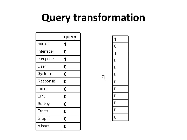
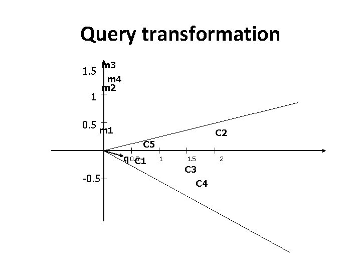
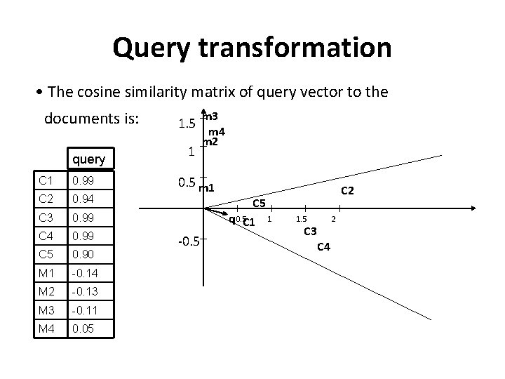
LSI Example • Query: “human computer interaction” retrieves documents: c 1, c 2, c 4 but not c 3 and c 5. • If we submit the same query (based on the transformation shown before) to the transformed matrix we retrieve (using cosine similarity) all c 1 -c 5 even if c 3 and c 5 have no common keyword to the query. • According to the transformation for the queries we have:

Query transformation query 1 human 1 0 Interface 0 1 computer 1 0 User 0 0 System 0 Response 0 Time 0 0 EPS 0 0 Survey 0 0 Trees 0 0 Graph 0 0 Minors 0 q= 0 0

Query transformation q T= U k= 1 0 0. 22 -0. 11 0. 20 -0. 07 0. 24 0. 04 0. 40 0. 06 0. 64 -0. 17 0. 27 0. 11 0. 30 -0. 14 0. 21 0. 27 0. 01 0. 49 0. 04 0. 62 0. 03 0. 45 1 0 0 0 Lk= qn=q. TUk. Lk = 0 0. 3 0 0 0. 39 0. 138 0 0 -0. 0273 0

Query transformation Map docs to the 2 dim space Vk. Lk= q n. L k = 0. 20 -0. 06 0. 67 -0. 15 0. 61 0. 17 2. 04 0. 43 0. 46 -0. 13 1. 54 -0. 33 0. 54 -0. 23 1. 80 -0. 58 0. 28 0. 11 0. 94 0. 28 0. 00 0. 19 0. 00 0. 48 0. 01 0. 44 0. 03 1. 12 0. 02 0. 62 0. 07 1. 57 0. 08 0. 53 0. 27 1. 35 0. 138 3. 34 0 0 2. 54 -0. 0273 = 3. 34 0 0 2. 54 = 0. 46 -0. 069

Query transformation 1. 5 1 m 3 m 4 m 2 0. 5 m 1 C 2 C 5 q 0. 5 C 1 -0. 5 1 1. 5 2 C 3 C 4

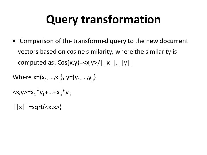
Query transformation • Comparison of the transformed query to the new document vectors based on cosine similarity, where the similarity is computed as: Cos(x, y)=<x, y>/||x||. ||y|| Where x=(x 1, …, xn), y=(y 1, …, yn) <x, y>=x 1*y 1+…+xn*yn ||x||=sqrt(<x, x>)

Query transformation • The cosine similarity matrix of query vector to the documents is: query C 1 0. 99 C 2 0. 94 C 3 0. 99 C 4 0. 99 C 5 0. 90 M 1 -0. 14 M 2 -0. 13 M 3 -0. 11 M 4 0. 05 1. 5 1 m 3 m 4 m 2 0. 5 m 1 C 5 q 0. 5 C 1 1 -0. 5 C 2 1. 5 2 C 3 C 4