Feature Selection Section 4 2 from Jain A

Feature Selection Section 4. 2 from Jain, A. K. ; Duin, P. W. ; Jianchang Mao, “Statistical pattern recognition: a review”, IEEE Transactions on Pattern Analysis and Machine Intelligence, vol. 22, no. 1, pp. 4 -37, Jan. 2000. & Section 4. 2 from textbook Genetic Algorithms Section 7. 5 from textbook CS 479/679 Pattern Recognition Dr. George Bebis

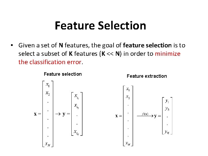
Feature Selection • Given a set of N features, the goal of feature selection is to select a subset of K features (K << N) in order to minimize the classification error. Feature selection Feature extraction

Feature Selection vs Feature Extraction • Feature Extraction – New features are combinations (linear for PCA/LDA) of the original features (difficult to interpret). – When classifying novel patterns, all features need to be computed. • Feature Selection – New features represent a subset of the original features. – When classifying novel patterns, only a small number of features need to be computed (i. e. , faster classification).

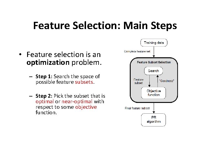
Feature Selection: Main Steps • Feature selection is an optimization problem. – Step 1: Search the space of possible feature subsets. – Step 2: Pick the subset that is optimal or near-optimal with respect to some objective function.

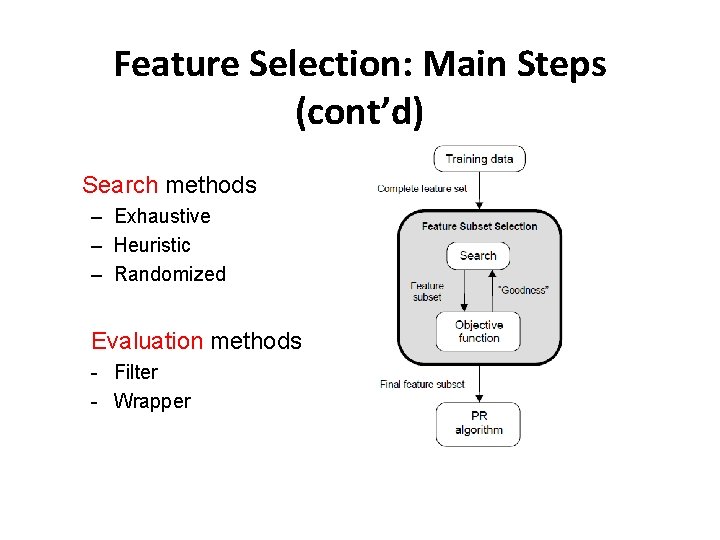
Feature Selection: Main Steps (cont’d) Search methods – Exhaustive – Heuristic – Randomized Evaluation methods - Filter - Wrapper

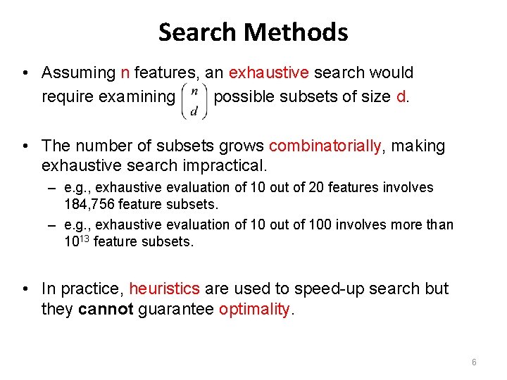
Search Methods • Assuming n features, an exhaustive search would require examining possible subsets of size d. • The number of subsets grows combinatorially, making exhaustive search impractical. – e. g. , exhaustive evaluation of 10 out of 20 features involves 184, 756 feature subsets. – e. g. , exhaustive evaluation of 10 out of 100 involves more than 1013 feature subsets. • In practice, heuristics are used to speed-up search but they cannot guarantee optimality. 6

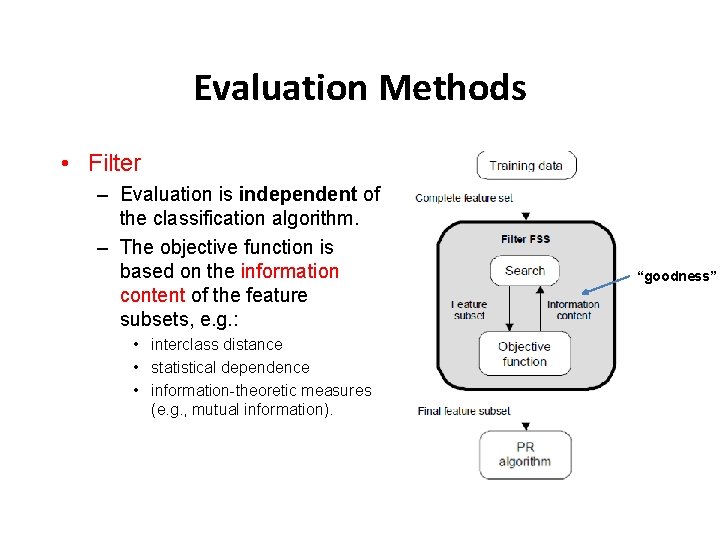
Evaluation Methods • Filter – Evaluation is independent of the classification algorithm. – The objective function is based on the information content of the feature subsets, e. g. : • interclass distance • statistical dependence • information-theoretic measures (e. g. , mutual information). “goodness”

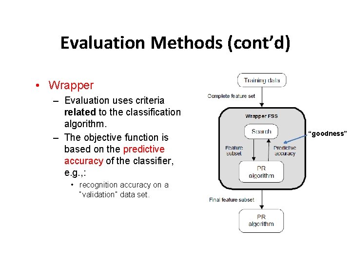
Evaluation Methods (cont’d) • Wrapper – Evaluation uses criteria related to the classification algorithm. – The objective function is based on the predictive accuracy of the classifier, e. g. , : • recognition accuracy on a “validation” data set. “goodness”

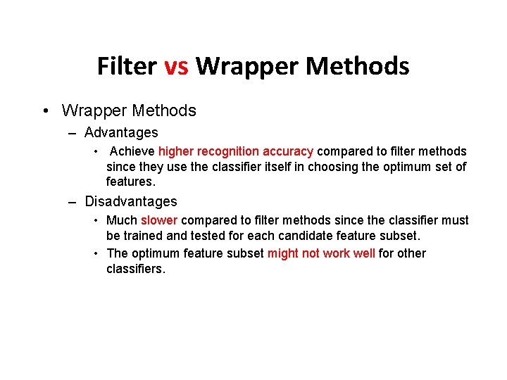
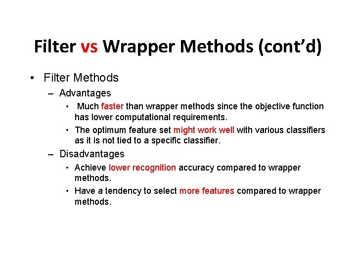
Filter vs Wrapper Methods • Wrapper Methods – Advantages • Achieve higher recognition accuracy compared to filter methods since they use the classifier itself in choosing the optimum set of features. – Disadvantages • Much slower compared to filter methods since the classifier must be trained and tested for each candidate feature subset. • The optimum feature subset might not work well for other classifiers.

Filter vs Wrapper Methods (cont’d) • Filter Methods – Advantages Much faster than wrapper methods since the objective function has lower computational requirements. • The optimum feature set might work well with various classifiers as it is not tied to a specific classifier. • – Disadvantages • Achieve lower recognition accuracy compared to wrapper methods. • Have a tendency to select more features compared to wrapper methods.

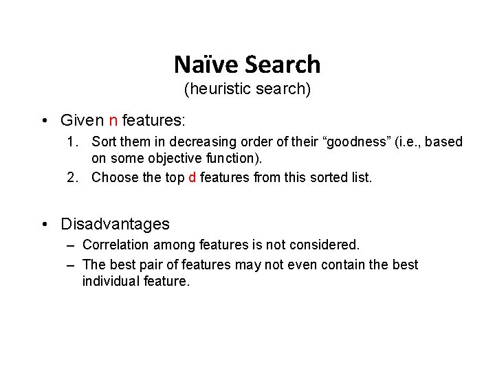
Naïve Search (heuristic search) • Given n features: 1. Sort them in decreasing order of their “goodness” (i. e. , based on some objective function). 2. Choose the top d features from this sorted list. • Disadvantages – Correlation among features is not considered. – The best pair of features may not even contain the best individual feature.

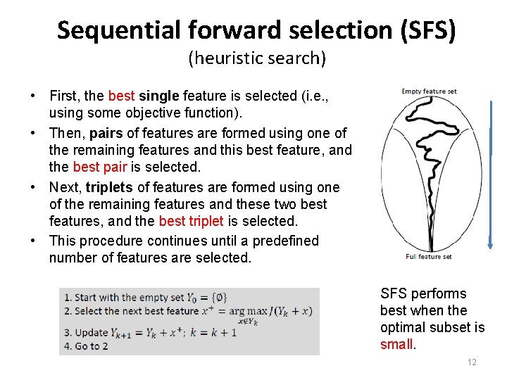
Sequential forward selection (SFS) (heuristic search) • First, the best single feature is selected (i. e. , using some objective function). • Then, pairs of features are formed using one of the remaining features and this best feature, and the best pair is selected. • Next, triplets of features are formed using one of the remaining features and these two best features, and the best triplet is selected. • This procedure continues until a predefined number of features are selected. SFS performs best when the optimal subset is small. 12

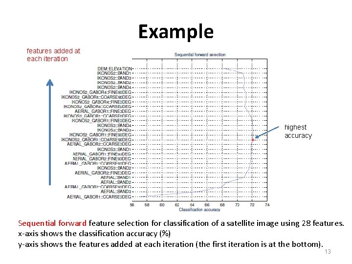
Example features added at each iteration highest accuracy Sequential forward feature selection for classification of a satellite image using 28 features. x-axis shows the classification accuracy (%) y-axis shows the features added at each iteration (the first iteration is at the bottom). 13

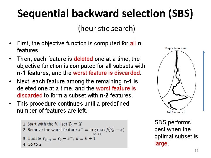
Sequential backward selection (SBS) (heuristic search) • First, the objective function is computed for all n features. • Then, each feature is deleted one at a time, the objective function is computed for all subsets with n-1 features, and the worst feature is discarded. • Next, each feature among the remaining n-1 is deleted one at a time, and the worst feature is discarded to form a subset with n-2 features. • This procedure continues until a predefined number of features are left. SBS performs best when the optimal subset is large. 14

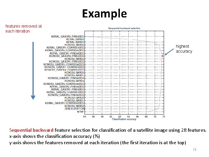
Example features removed at each iteration highest accuracy Sequential backward feature selection for classification of a satellite image using 28 features. x-axis shows the classification accuracy (%) y-axis shows the features removed at each iteration (the first iteration is at the top) 15

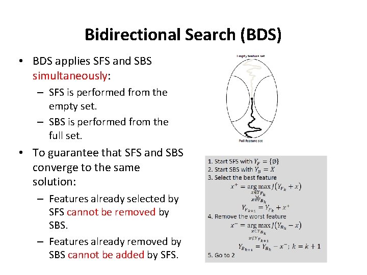
Bidirectional Search (BDS) • BDS applies SFS and SBS simultaneously: – SFS is performed from the empty set. – SBS is performed from the full set. • To guarantee that SFS and SBS converge to the same solution: – Features already selected by SFS cannot be removed by SBS. – Features already removed by SBS cannot be added by SFS. Y

Limitations of SFS and SBS • The main limitation of SFS is that it is unable to remove features that become non useful after the addition of other features. • The main limitation of SBS is its inability to reevaluate the usefulness of a feature after it has been discarded. • Enhancements of SFS and SBS: – “Plus-L, minus-R” selection (LRS) – Sequential floating forward (or backward) selection (i. e. , SFFS and SFBS)

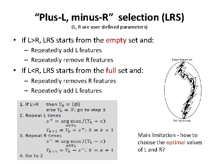
“Plus-L, minus-R” selection (LRS) (L, R are user-defined parameters) • If L>R, LRS starts from the empty set and: – Repeatedly add L features – Repeatedly remove R features • If L<R, LRS starts from the full set and: – Repeatedly removes R features – Repeatedly add L features Main limitation - how to choose the optimal values of L and R?

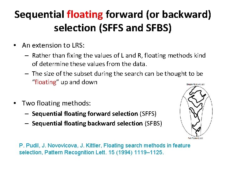
Sequential floating forward (or backward) selection (SFFS and SFBS) • An extension to LRS: – Rather than fixing the values of L and R, floating methods kind of determine these values from the data. – The size of the subset during the search can be thought to be “floating” up and down • Two floating methods: – Sequential floating forward selection (SFFS) – Sequential floating backward selection (SFBS) P. Pudil, J. Novovicova, J. Kittler, Floating search methods in feature selection, Pattern Recognition Lett. 15 (1994) 1119– 1125.

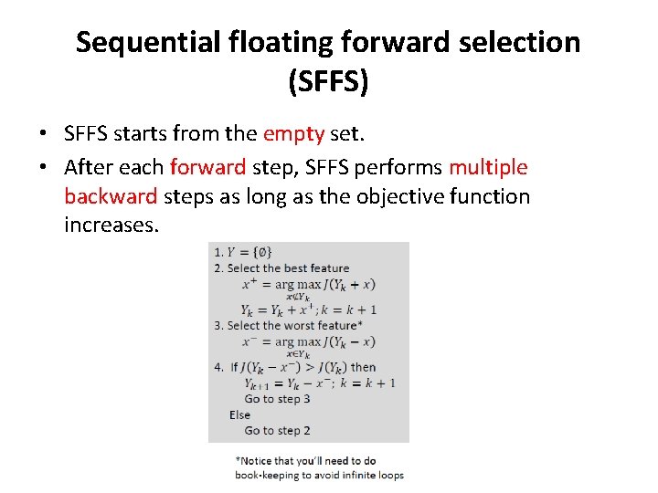
Sequential floating forward selection (SFFS) • SFFS starts from the empty set. • After each forward step, SFFS performs multiple backward steps as long as the objective function increases.

Sequential floating backward selection (SFBS) • Sequential floating backward selection (SFBS) starts from the full set. • After each backward step, SFBS performs multiple forward steps as long as the objective function increases.

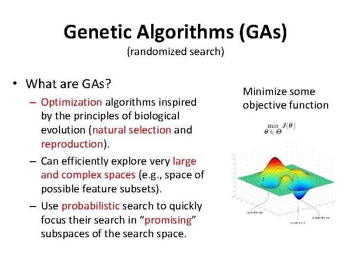
Genetic Algorithms (GAs) (randomized search) • What are GAs? – Optimization algorithms inspired by the principles of biological evolution (natural selection and reproduction). – Can efficiently explore very large and complex spaces (e. g. , space of possible feature subsets). – Use probabilistic search to quickly focus their search in “promising” subspaces of the search space. Minimize some objective function

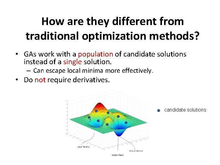
How are they different from traditional optimization methods? • GAs work with a population of candidate solutions instead of a single solution. – Can escape local minima more effectively. • Do not require derivatives. candidate solutions

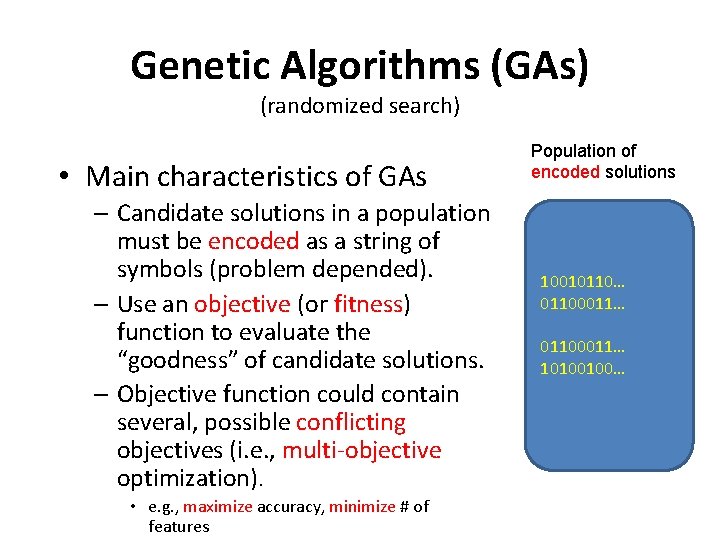
Genetic Algorithms (GAs) (randomized search) • Main characteristics of GAs – Candidate solutions in a population must be encoded as a string of symbols (problem depended). – Use an objective (or fitness) function to evaluate the “goodness” of candidate solutions. – Objective function could contain several, possible conflicting objectives (i. e. , multi-objective optimization). • e. g. , maximize accuracy, minimize # of features Population of encoded solutions 10010110… 01100011… 10100100…

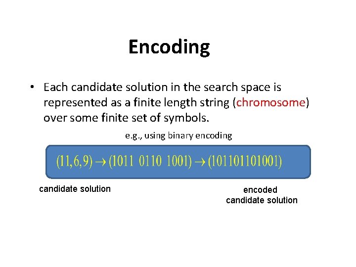
Encoding • Each candidate solution in the search space is represented as a finite length string (chromosome) over some finite set of symbols. e. g. , using binary encoding candidate solution encoded candidate solution

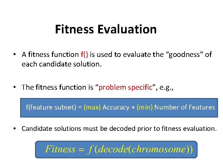
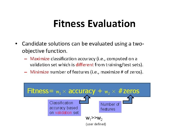
Fitness Evaluation • A fitness function f() is used to evaluate the “goodness” of each candidate solution. • The fitness function is “problem specific”, e. g. , f(feature subset) = (max) Accuracy + (min) Number of Features • Candidate solutions must be decoded prior to fitness evaluation.

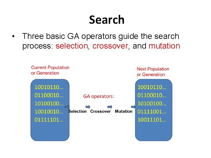
Search • Three basic GA operators guide the search process: selection, crossover, and mutation

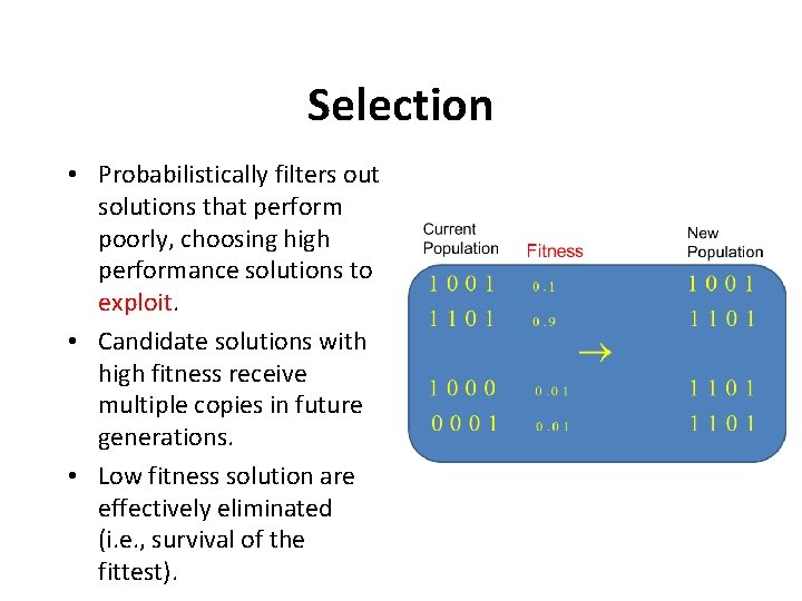
Selection • Probabilistically filters out solutions that perform poorly, choosing high performance solutions to exploit. • Candidate solutions with high fitness receive multiple copies in future generations. • Low fitness solution are effectively eliminated (i. e. , survival of the fittest).

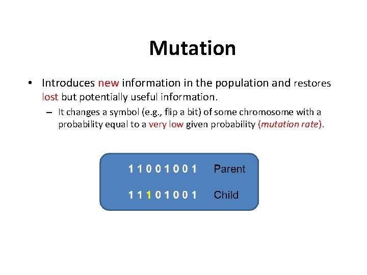
Mutation • Introduces new information in the population and restores lost but potentially useful information. – It changes a symbol (e. g. , flip a bit) of some chromosome with a probability equal to a very low given probability (mutation rate).

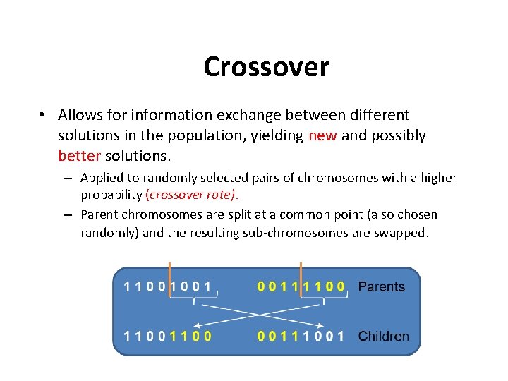
Crossover • Allows for information exchange between different solutions in the population, yielding new and possibly better solutions. – Applied to randomly selected pairs of chromosomes with a higher probability (crossover rate). – Parent chromosomes are split at a common point (also chosen randomly) and the resulting sub-chromosomes are swapped.

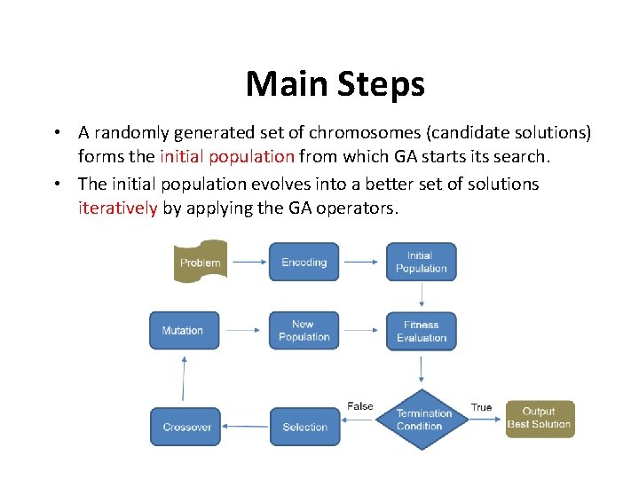
Main Steps • A randomly generated set of chromosomes (candidate solutions) forms the initial population from which GA starts its search. • The initial population evolves into a better set of solutions iteratively by applying the GA operators.

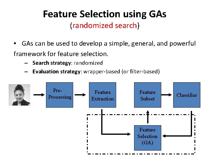
Feature Selection using GAs (randomized search) • GAs can be used to develop a simple, general, and powerful framework for feature selection. – Search strategy: randomized – Evaluation strategy: wrapper-based (or filter-based) Pre. Processing Feature Extraction Feature Subset Feature Selection (GA) Classifier

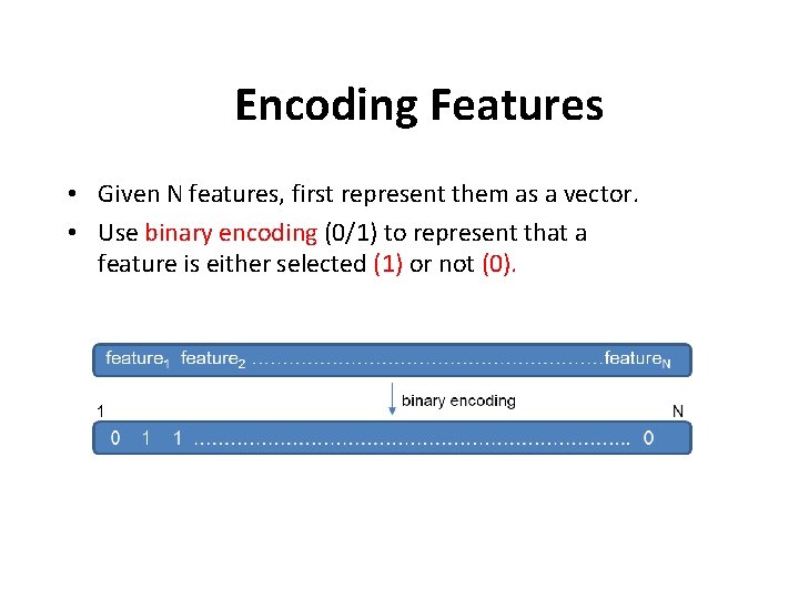
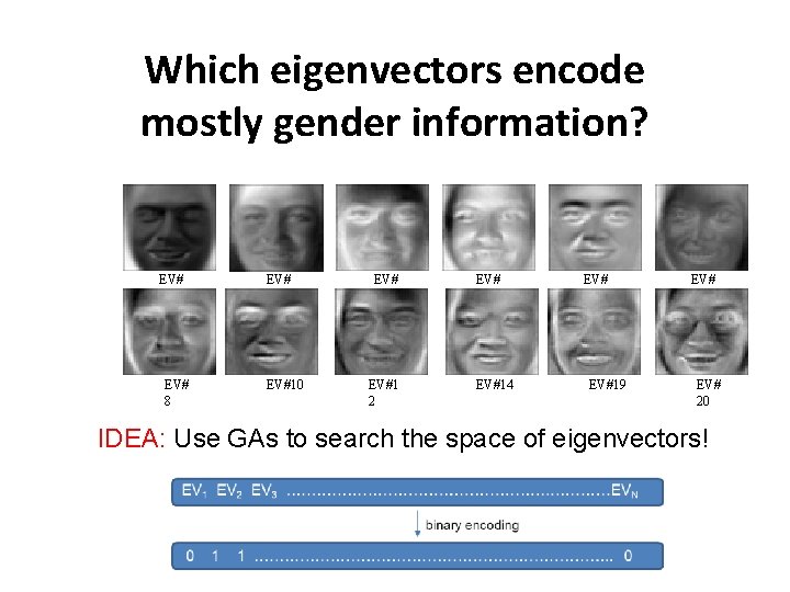
Encoding Features • Given N features, first represent them as a vector. • Use binary encoding (0/1) to represent that a feature is either selected (1) or not (0).

Fitness Evaluation • Candidate solutions can be evaluated using a twoobjective function. – Maximize classification accuracy (i. e. , computed on a validation set which is different from training/test sets). – Minimize number of features (i. e. , maximize # of zeros). Fitness= w 1 accuracy + Classification accuracy based on validation set w 2 #zeros Number of features w 1>>w 2 (user defined)

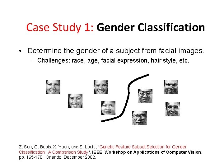
Case Study 1: Gender Classification • Determine the gender of a subject from facial images. – Challenges: race, age, facial expression, hair style, etc. Z. Sun, G. Bebis, X. Yuan, and S. Louis, "Genetic Feature Subset Selection for Gender Classification: A Comparison Study", IEEE Workshop on Applications of Computer Vision, pp. 165 -170, Orlando, December 2002.

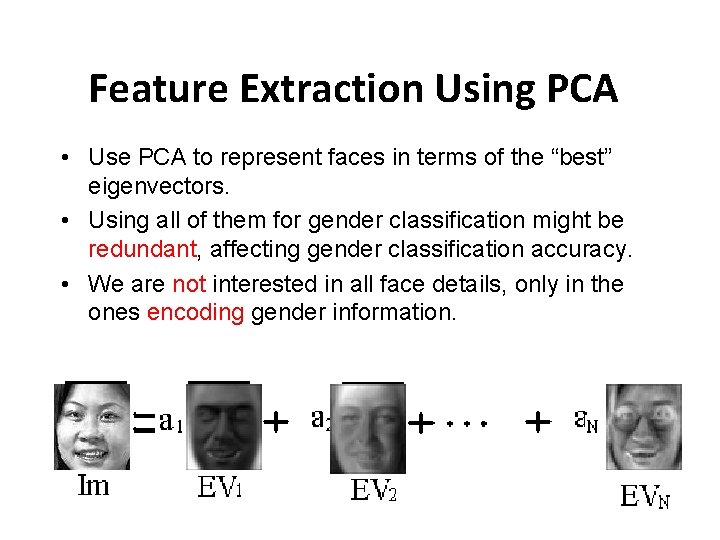
Feature Extraction Using PCA • Use PCA to represent faces in terms of the “best” eigenvectors. • Using all of them for gender classification might be redundant, affecting gender classification accuracy. • We are not interested in all face details, only in the ones encoding gender information.

Which eigenvectors encode mostly gender information? EV# 1 EV# 8 EV# 2 EV#10 EV# 3 EV#1 2 EV# 4 EV#14 EV# 5 EV#19 EV# 6 EV# 20 IDEA: Use GAs to search the space of eigenvectors!

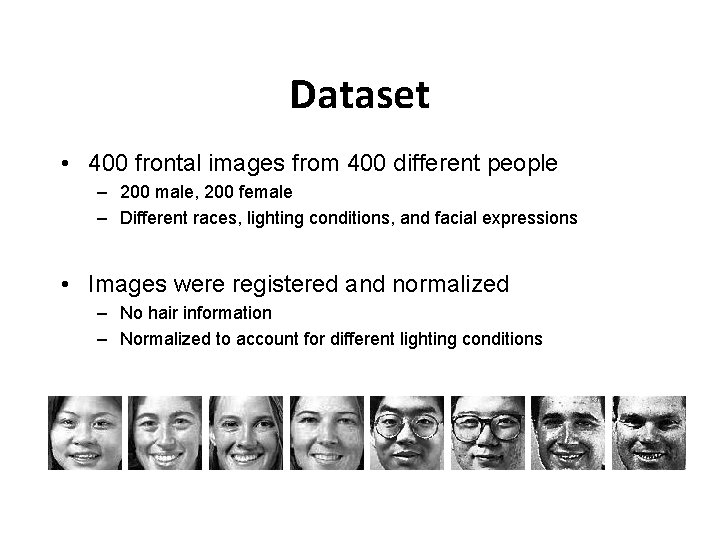
Dataset • 400 frontal images from 400 different people – 200 male, 200 female – Different races, lighting conditions, and facial expressions • Images were registered and normalized – No hair information – Normalized to account for different lighting conditions

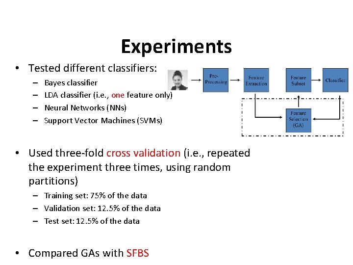
Experiments • Tested different classifiers: – – Bayes classifier LDA classifier (i. e. , one feature only) Neural Networks (NNs) Support Vector Machines (SVMs) • Used three-fold cross validation (i. e. , repeated the experiment three times, using random partitions) – Training set: 75% of the data – Validation set: 12. 5% of the data – Test set: 12. 5% of the data • Compared GAs with SFBS

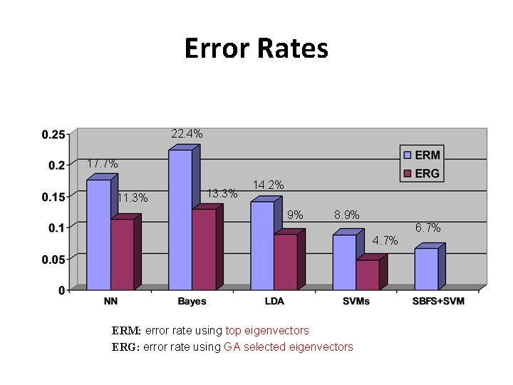
Error Rates 22. 4% 17. 7% 11. 3% 13. 3% 14. 2% 9% 8. 9% 6. 7% 4. 7% ERM: error rate using top eigenvectors ERG: error rate using GA selected eigenvectors

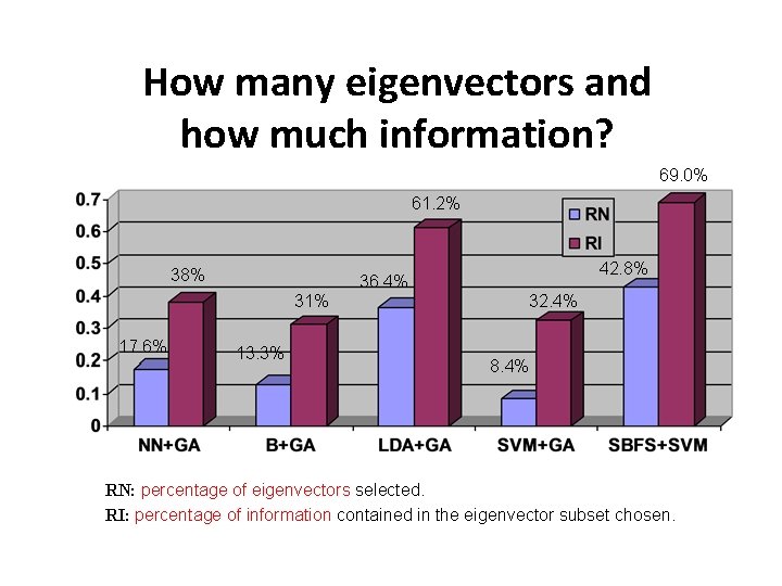
How many eigenvectors and how much information? 69. 0% 61. 2% 38% 31% 17. 6% 42. 8% 36. 4% 13. 3% 32. 4% 8. 4% RN: percentage of eigenvectors selected. RI: percentage of information contained in the eigenvector subset chosen.

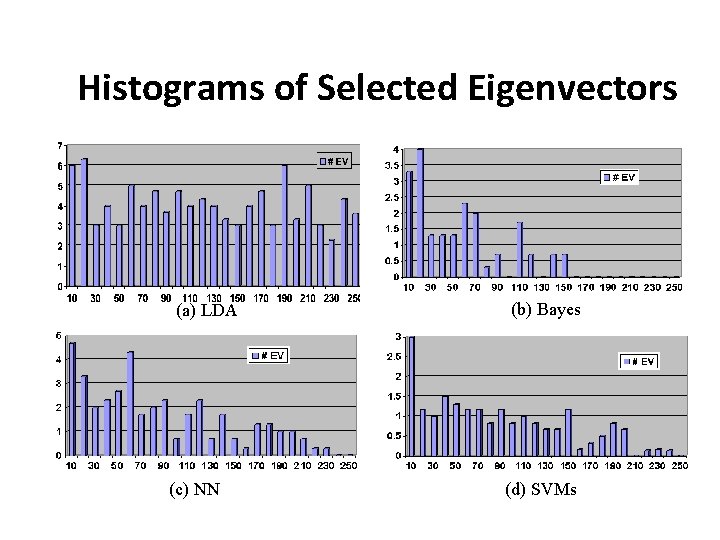
Histograms of Selected Eigenvectors (a) LDA (c) NN (b) Bayes (d) SVMs

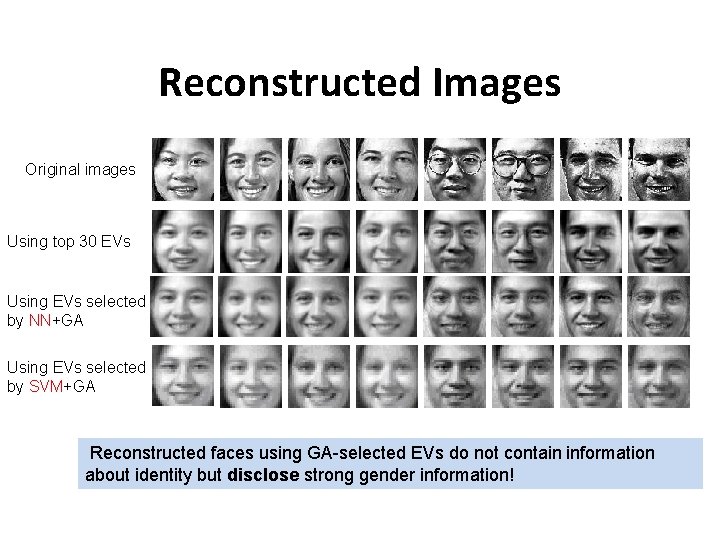
Reconstructed Images Original images Using top 30 EVs Using EVs selected by NN+GA Using EVs selected by SVM+GA Reconstructed faces using GA-selected EVs do not contain information about identity but disclose strong gender information!

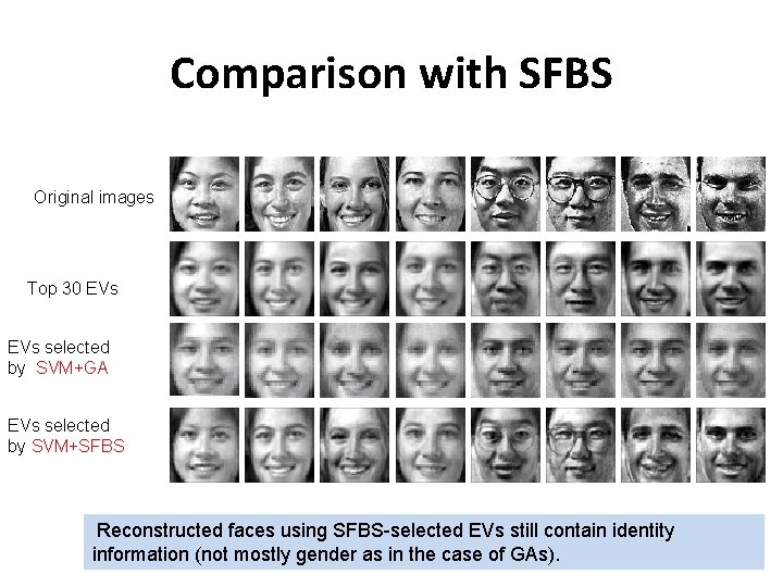
Comparison with SFBS Original images Top 30 EVs selected by SVM+GA EVs selected by SVM+SFBS Reconstructed faces using SFBS-selected EVs still contain identity information (not mostly gender as in the case of GAs).

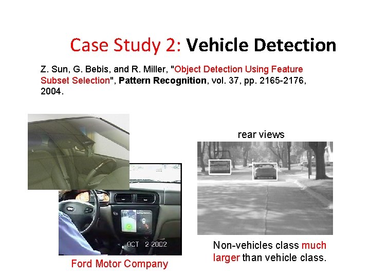
Case Study 2: Vehicle Detection Z. Sun, G. Bebis, and R. Miller, "Object Detection Using Feature low light camera Subset Selection", Pattern Recognition, vol. 37, pp. 2165 -2176, 2004. rear views Ford Motor Company Non-vehicles class much larger than vehicle class.

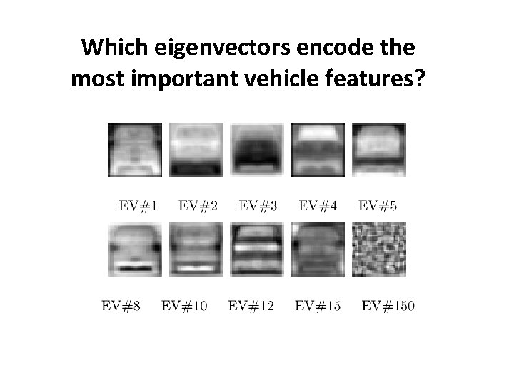
Which eigenvectors encode the most important vehicle features?

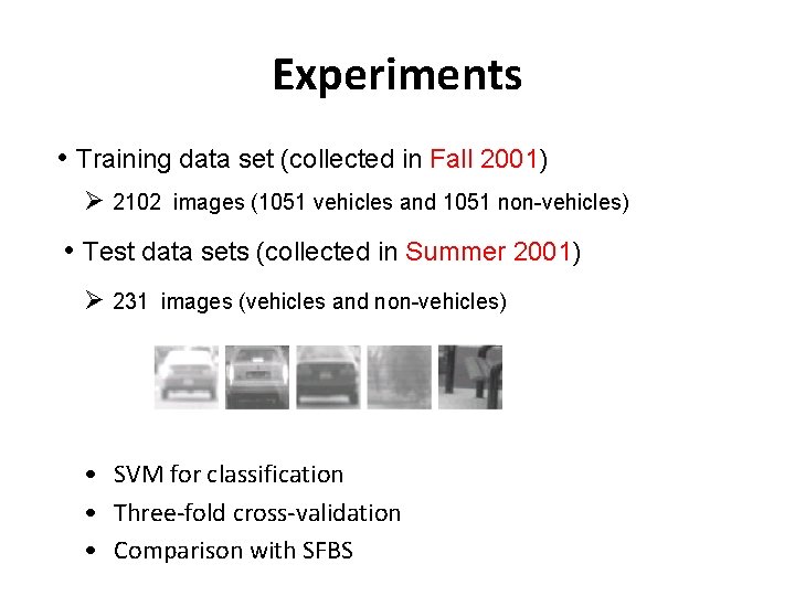
Experiments • Training data set (collected in Fall 2001) Ø 2102 images (1051 vehicles and 1051 non-vehicles) • Test data sets (collected in Summer 2001) Ø 231 images (vehicles and non-vehicles) • SVM for classification • Three-fold cross-validation • Comparison with SFBS

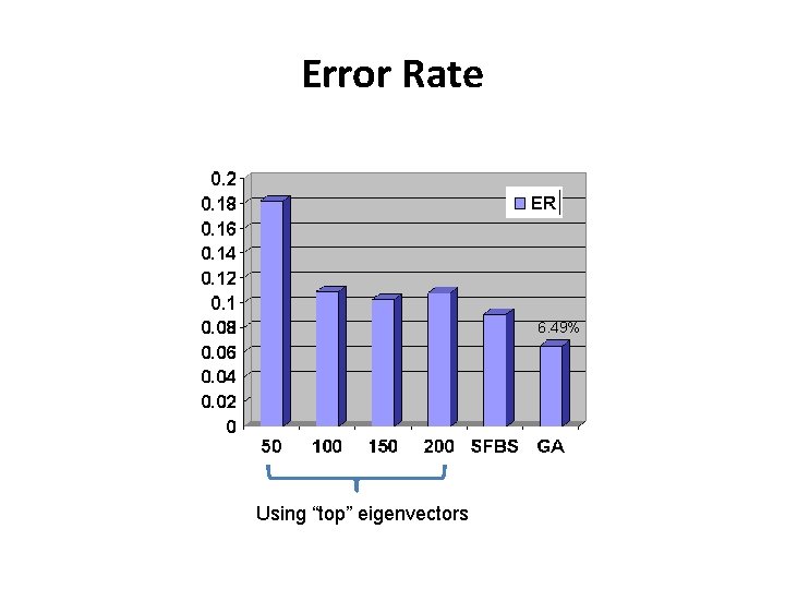
Error Rate 6. 49% Using “top” eigenvectors

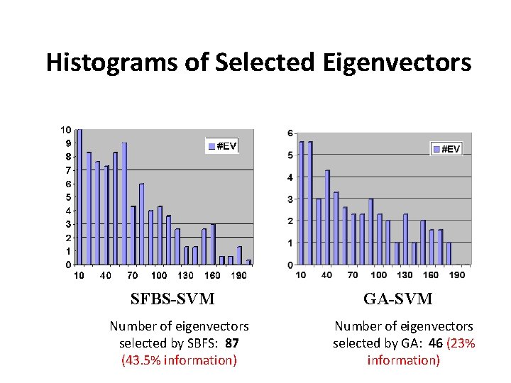
Histograms of Selected Eigenvectors SFBS-SVM Number of eigenvectors selected by SBFS: 87 (43. 5% information) GA-SVM Number of eigenvectors selected by GA: 46 (23% information)

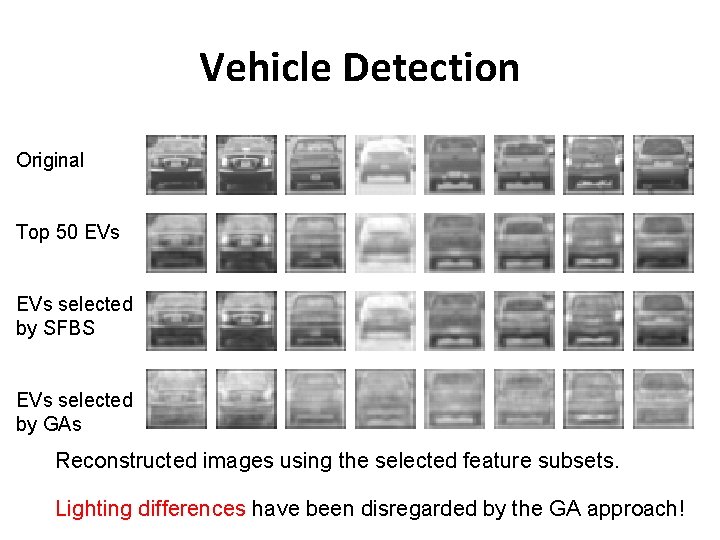
Vehicle Detection Original Top 50 EVs selected by SFBS EVs selected by GAs Reconstructed images using the selected feature subsets. Lighting differences have been disregarded by the GA approach!

Case Study 3: Fusion of Visible-Thermal IR Imagery for Face Recognition • Improve face recognition performance by integrating information both from the visible and infrared spectrum. G. Bebis, A. Gyaourova, S. Singh, and I. Pavlidis, "Face Recognition by Fusing Thermal Infrared and Visible Imagery", Image and Vision Computing, vol. 24, no. 7, pp. 727 -742, 2006.

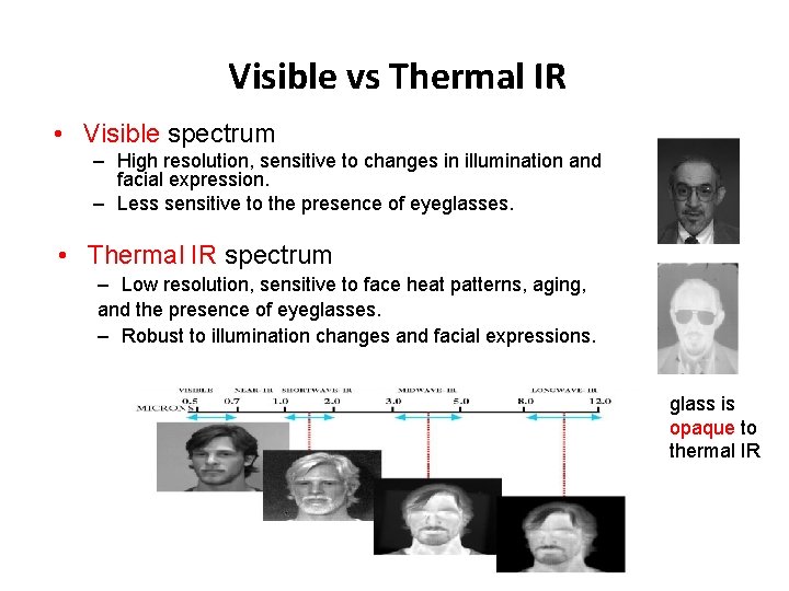
Visible vs Thermal IR • Visible spectrum – High resolution, sensitive to changes in illumination and facial expression. – Less sensitive to the presence of eyeglasses. • Thermal IR spectrum – Low resolution, sensitive to face heat patterns, aging, and the presence of eyeglasses. – Robust to illumination changes and facial expressions. glass is opaque to thermal IR

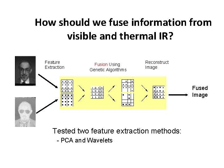
How should we fuse information from visible and thermal IR? Feature Extraction Fusion Using Genetic Algorithms Reconstruct Image Fused Image Tested two feature extraction methods: - PCA and Wavelets

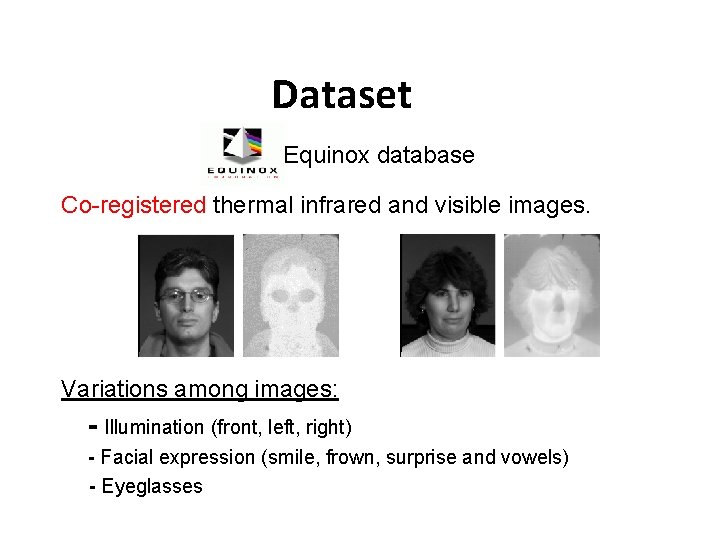
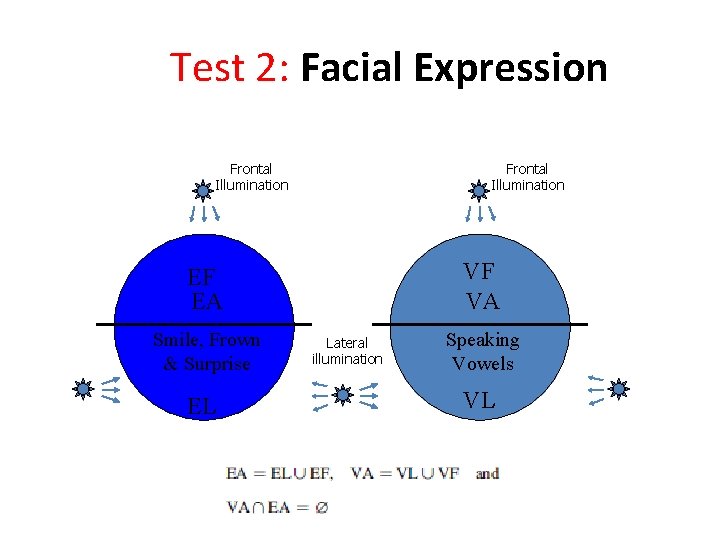
Dataset Equinox database Co-registered thermal infrared and visible images. Variations among images: - Illumination (front, left, right) - Facial expression (smile, frown, surprise and vowels) - Eyeglasses

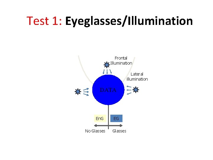
Test 1: Eyeglasses/Illumination Frontal Illumination EFn. G EFG DATA ELn. G En. G No Glasses ELG EG Glasses Lateral illumination

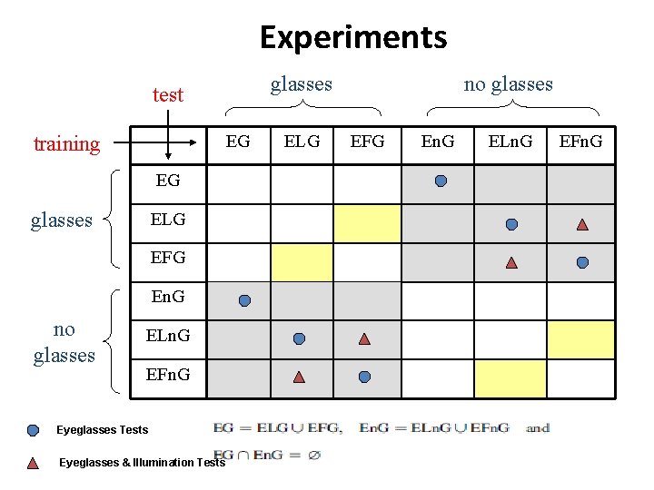
Experiments glasses test EG training EG glasses ELG EFG En. G no glasses ELn. G EFn. G Eyeglasses Tests Eyeglasses & Illumination Tests ELG no glasses EFG En. G ELn. G EFn. G

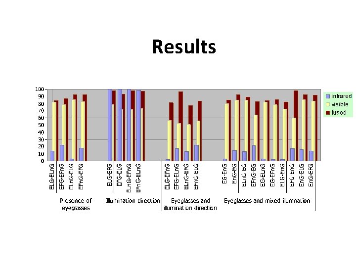
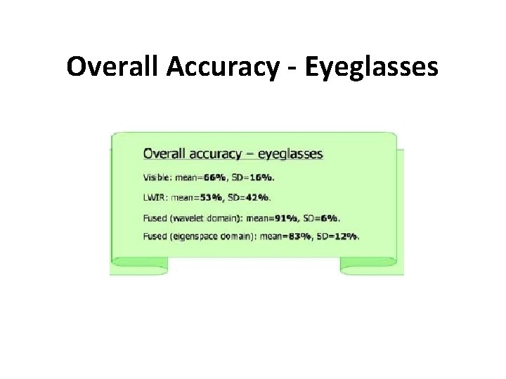
Results

Overall Accuracy - Eyeglasses

Test 2: Facial Expression Frontal Illumination VF VA EF EA Smile, Frown & Surprise EL Lateral illumination Speaking Vowels VL

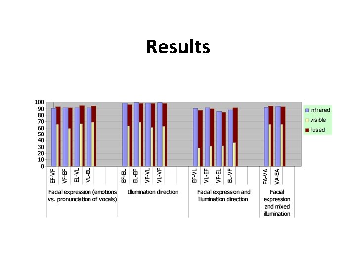
Results

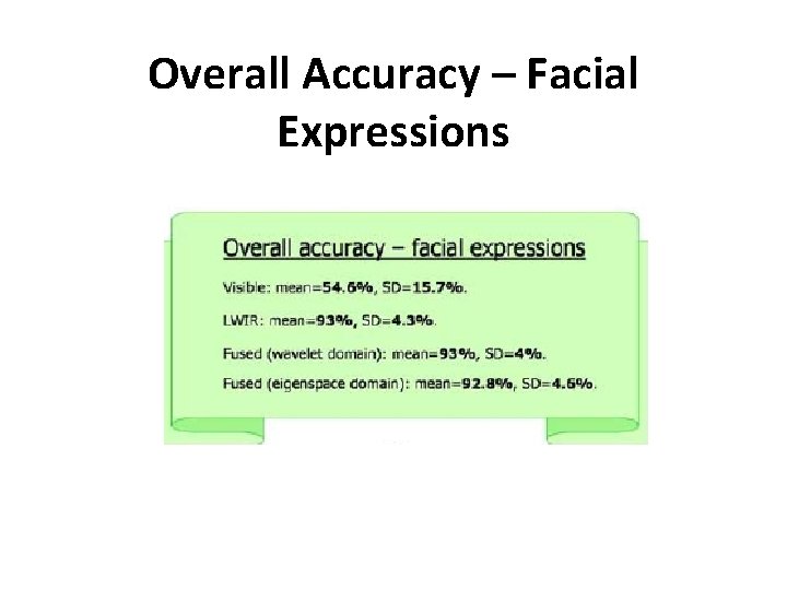
Overall Accuracy – Facial Expressions

Next Quiz • When: Thursday, April 9 th • What: Feature Selection