Dimensionality Reduction Thomas Schwarz SJ Introduction Feature selection

Dimensionality Reduction Thomas Schwarz, SJ

Introduction • Feature selection • Data sets contain often large numbers of features • • Some of the features depend on each other Selecting features • • • makes current classification fast can generalize better from training to general data This even works with Neural Networks

Introduction • Feature Combination: • Generate artificial features by combining features • Then do away with (some of the) old features

Introduction • Clustering: • Automatic clustering • Groups similar data points • Often allows fewer features to be used

Introduction • Automatic dimensionality reduction: • Project 2 -dimensional data set on a single line • Projections separates the two data sets • Can use a single, combined feature for classification • Linear Discriminant Analysis

Introduction • Two-dimensional data set • • Spread around one dimension Combine the two features (x, y) into one that has almost all the variance • Principal component analysis

Principal Component Analysis • Goal: • Find the one direction in which the data sets varies most

Principal Component Analysis • • Given a set of of data points with numerical attributes Write as an matrix

Principal Component Analysis • Each data point is a linear combination of standard basis • Dimensionality reduction: • Replace standard basis with another orthogonal matrix • Weight of data should be concentrated in a few dimensions

Principal Component Analysis • Assume is such a basis • • Then Actually, any vectors of length one with this property are a basis Proof: If , then

Principal Component Analysis • Write the vectors in an orthonormal basis as column vectors of a matrix Then: implies:

Principal Component Analysis A feature vector is a linear combination. Write: Then or equivalently

Principal Component Analysis is an orthonormal basis of Matrix is

Principal Component Analysis Column vector is a linear combination of the column vectors of. Use Multiply with Obtain:

Principal Component Analysis: Projection on Subspace Write a data point as Assume that we have ordered the basis by importance We select only the first components: Write: Then set

Principal Component Analysis: Projection on Subspace Since , it follows and is called the projection matrix since (a) (b)

Principal Component Analysis: Projection on Subspace Example (continued): Project on the first two coordinates with respect to

Principal Component Analysis: Projection on Subspace Then we calculate the projection matrix

Principal Component Analysis: Projection on Subspace Projection of is

Principal Component Analysis: Projection on Subspace • Now we know how to project • Need to find the best orthonormal matrix for the projection

Single Principal Component Analysis • • • There are infinitely many choices of orthonormal bases Start out with reduction to a single dimension First step: Center the data set • • By subtracting the mean of the data set Therefore: The mean of the data set is zero

Single Principal Component Analysis • If we reduce to a single dimension, than the partial basis is given by a single vector. • Optimality criterion: Projection maximizes the variance

Single Principal Component Analysis

Single Principal Component Analysis • Therefore: • Use Lagrange multiplier and now maximize • So, we differentiate: subject to

Single Principal Component Analysis • • Result: Maximum obtained if • And to maximize, we want the eigenvector with the largest eigenvalue With other words: eigenvalue. has to be an eigenvector of with

Single Principal Component Analysis • Turns out that finding the maximum eigenvector and eigenvalue is quite simple: • Write any non-zero vector as a combination of eigenvectors • Then repeatedly apply the matrix, but always normalize the product • The coefficient corresponding to the largest eigenvalue gets more and more magnified • And in the limit, the product will be the eigenvector corresponding to the largest eigenvalue

Single Principal Component Analysis • Another goodness criterion: • Minimize the sum of squares of the differences between projected values and original values of the feature vector • Error is

Single Principal Component Analysis

Single Principal Component Analysis • This means: • • • In order to minimize the sum of squared errors, Need to minimize the projected variance Our two criteria are the same

Dual Principal Component Analysis • • • We can redo our calculation for two dimensions • Need to pick the two eigenvectors with the two largest eigenvalues Calculate just as before the minimum variance Obtain: minimum variance is the sum of the two largest eigenvalues

PCA in Python • Part of sklearn. decomposition • Import bunch of modules import numpy as np import matplotlib. pyplot as plt import seaborn as sns from sklearn. decomposition import PCA • Create random, but skewed data set , rng = np. random. Random. State(2020716) X = np. dot(rng. rand(2, 2), rng. randn(2, 200)). T

PCA in Python • Here is some code to draw a vector def draw_vector(v 0, v 1, ax=None): ax = ax or plt. gca() arrowprops=dict(arrowstyle='->', linewidth=1, shrink. A=0, shrink. B=0) ax. annotate('', v 1, v 0, arrowprops=arrowprops)

PCA in Python • Calculate the PCA (with two components) pca = PCA(n_components=2) pca. fit(X) print(pca. components_) print(pca. explained_variance_)

PCA in Python • First component has almost all the variance: [[-0. 99638832 -0. 08491358] [-0. 08491358 0. 99638832]] [0. 89143208 0. 01057402]

PCA in Python • Draw everything: plt. scatter(X[: , 0], X[: , 1], s=2, c='blue') for length, vector in zip(pca. explained_variance_, pc v = vector * 2. 3 * np. sqrt(length) draw_vector(pca. mean_, pca. mean_ + v) plt. axis('equal') plt. show()

PCA in Python

PCA in Python • Can express data points in the new coordinates: pca = PCA(n_components=2, whiten=True) pca. fit(X) X_pca = pca. transform(X)

PCA in Python

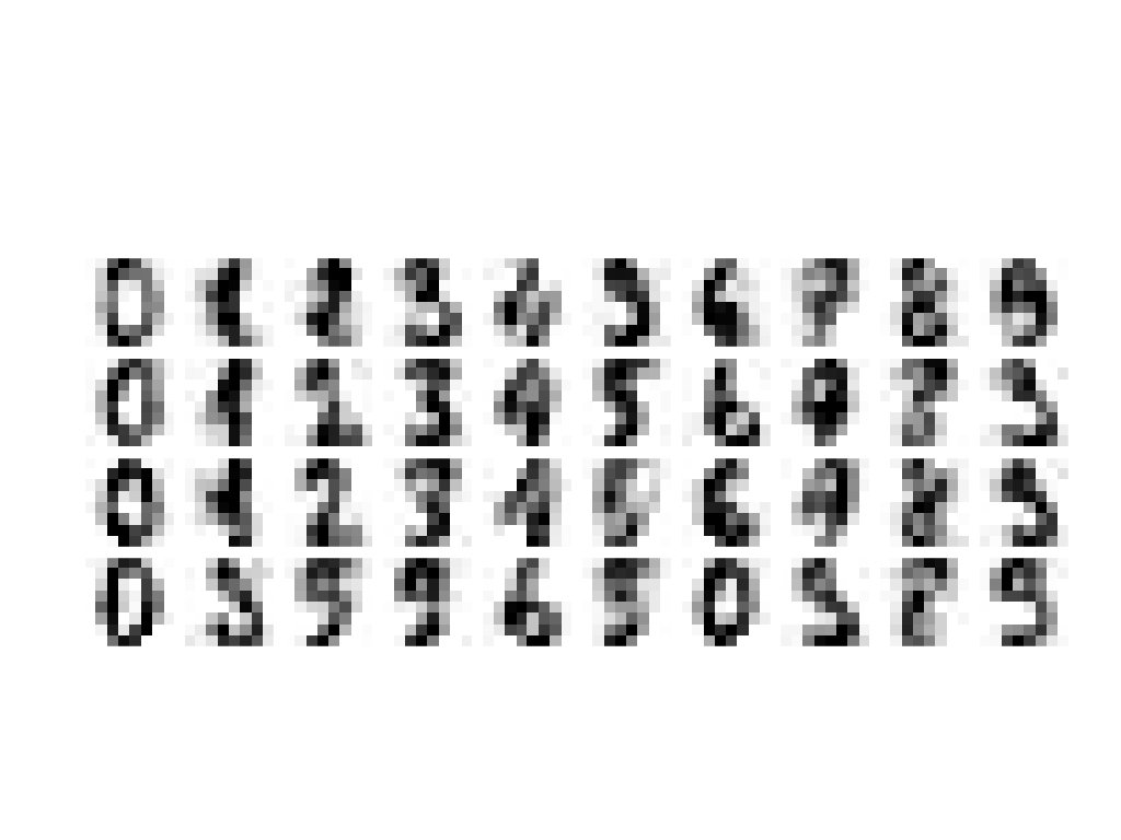
PCA in Python • Sklearn has the digit data-set • Used for learning how to recognize digits for post-office automation, etc

PCA in Python • Images have 64 pixels with gray values from sklearn. datasets import load_digits = load_digits() >>> digits. data. shape (1797, 64)

PCA in Python • Can use PCA to lower dimension to two pca = PCA(2) projected = pca. fit_transform(digits. data)

PCA in Python • And display with the Spectral colormap plt. scatter(projected[: , 0], projected[: , 1], s=5, c=digits. target, edgecolor='none', alpha=0. 7, cmap=plt. cm. get_cmap('Spectral', 10)) plt. xlabel('component 1') plt. ylabel('component 2') plt. colorbar(); plt. show()

PCA in Python • Result shows that two features already give a decent classification:

PCA in Python

PCA in Python • We can calculate the complete orthonormal base • And decide how many features we might need by looking at the total explained variance pca = PCA(). fit(digits. data) plt. plot(np. cumsum(pca. explained_variance_ratio_)) plt. xlabel('number of components') plt. ylabel('cumulative explained variance') plt. show()

PCA in Python • Can also use this to filter noise: • Data will live primarily in the most important components

PCA in Python • Example: • Use some digits from the data set

PCA in Python • Now add some noise np. random. seed(42) noisy = np. random. normal(digits. data, 4) plot_digits(noisy)

PCA in Python

PCA in Python • Take the noisy set • Use enough components to obtain 50% explained variance pca = PCA(0. 50). fit(noisy) print(pca. n_components_) • Need 12 components in this case

PCA in Python • Then display the data of only the highest 12 components = pca. transform(noisy) filtered = pca. inverse_transform(components) plot_digits(filtered) plt. show()

PCA : Eigenfaces • There is a set of faces of important people in sklearn from sklearn. datasets import fetch_lfw_people sns. set() faces = fetch_lfw_people(min_faces_person=60) print(faces. target_names) print(faces. images. shape) ['Ariel Sharon' 'Colin Powell' 'Donald Rumsfeld' 'Geo 'Gerhard Schroeder' 'Hugo Chavez' 'Junichiro Koizumi (1348, 62, 47)

PCA : Eigenfaces • There is a randomized version of PCA that approximates • This is necessary because of the size of the data set pca = PCA(n_components=150, svd_solver = 'randomized', whiten=True ) pca. fit(faces. data)

pca = PCA(n_components=150, svd_solver = 'randomized', w pca. fit(faces. data) components = pca. transform(faces. data) projected = pca. inverse_transform(components) fig, ax = plt. subplots(2, 10, figsize=(10, 2. 5), subplot_kw={'xticks': [], 'yticks': []}, gridspec_kw=dict(hspace=0. 1, wspace=0. 1)) for i in range(10): ax[0, i]. imshow(faces. data[i]. reshape(62, 47), cmap= ax[1, i]. imshow(projected[i]. reshape(62, 47), cmap=' ax[0, 0]. set_ylabel('full-dimninput') ax[1, 0]. set_ylabel('150 -dimnreconstruction'); plt. show()

PCA : Eigenfaces • With about 150 components, the features of the faces are retained

Linear Discriminant Analysis • Idea: • • • Estimate mean and variance for each category Assumes same covariances Calculates (like PCA) an affine transformation

Linear Discriminant Analysis • Import LDA: from sklearn. discriminant_analysis import Linear. Discrim • Read data & divide iris = pd. read_csv('Iris. csv', index_col=0). drop(column X_train, X_test, y_train, y_test = train_test_split( iris, 50*[0]+50*[1]+50*[2], test_size=0. 2, random_state=0)

Linear Discriminant Analysis • Reset sc = Standard. Scaler() X_train = sc. fit_transform(X_train) X_test = sc. transform(X_test) • Train with two dimensions: lda = LDA(n_components=2) lda. fit(X_train, y_train) for i in range(len(X_test)): print(lda. predict([X_test[i]])[0], y_test[i])

Linear Discriminant Analysis • Results is 100%

Linear Discriminant Analysis • Show transformation for LDA: trans. X = lda. fit_transform(iris, 50*[0]+50*[1]+50*[2]) cmap = colors. Listed. Colormap(['b', 'r', 'g']) plt. scatter(trans. X[: , 0], trans. X[: , 1], s=3, c=50*[0]+50*[1]+50*[2], cmap = cmap ) plt. show()

Linear Discriminant Analysis