8 1 Inner Product Spaces Inner product Linear

8. 1. Inner Product Spaces Inner product Linear functional Adjoint

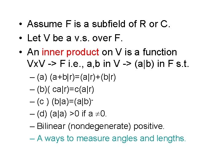
• Assume F is a subfield of R or C. • Let V be a v. s. over F. • An inner product on V is a function Vx. V -> F i. e. , a, b in V -> (a|b) in F s. t. – (a) (a+b|r)=(a|r)+(b|r) – (b)( ca|r)=c(a|r) – (c ) (b|a)=(a|b)– (d) (a|a) >0 if a 0. – Bilinear (nondegenerate) positive. – A ways to measure angles and lengths.

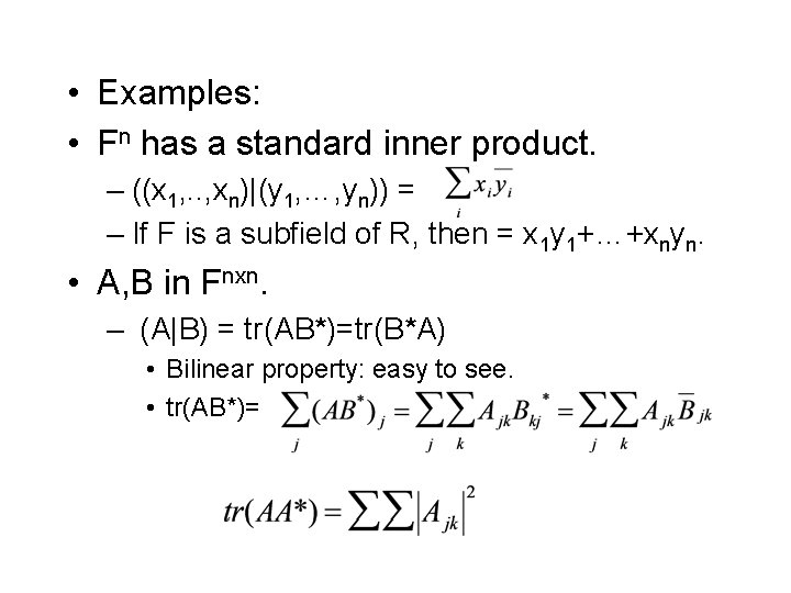
• Examples: • Fn has a standard inner product. – ((x 1, . . , xn)|(y 1, …, yn)) = – If F is a subfield of R, then = x 1 y 1+…+xnyn. • A, B in Fnxn. – (A|B) = tr(AB*)=tr(B*A) • Bilinear property: easy to see. • tr(AB*)=

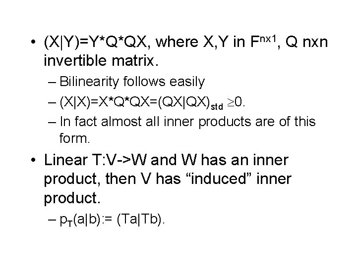
• (X|Y)=Y*Q*QX, where X, Y in Fnx 1, Q nxn invertible matrix. – Bilinearity follows easily – (X|X)=X*Q*QX=(QX|QX)std 0. – In fact almost all inner products are of this form. • Linear T: V->W and W has an inner product, then V has “induced” inner product. – p. T(a|b): = (Ta|Tb).

• (a) For any basis B={a 1, …, an}, there is an inner-product s. t. (ai|aj)= ij. – Define T: V->Fn s. t. ai -> ei. – Then p. T(ai|aj)=(ei|ej)= ij. • (b) V={f: [0, 1]->C| f is continuous }. – (f|g)= 01 fg- dt for f, g in V is an inner product. – T: V->V defined by f(t) -> tf(t) is linear. – p. T(f, g)= 01 tftg- dt= 01 t 2 fg- dt is an inner product.

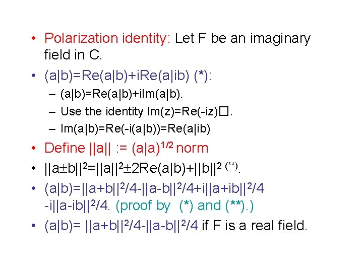
• Polarization identity: Let F be an imaginary field in C. • (a|b)=Re(a|b)+i. Re(a|ib) (*): – (a|b)=Re(a|b)+i. Im(a|b). – Use the identity Im(z)=Re(-iz)�. – Im(a|b)=Re(-i(a|b))=Re(a|ib) • Define ||a|| : = (a|a)1/2 norm • ||a b||2=||a||2 2 Re(a|b)+||b||2 (**). • (a|b)=||a+b||2/4 -||a-b||2/4+i||a+ib||2/4 -i||a-ib||2/4. (proof by (*) and (**). ) • (a|b)= ||a+b||2/4 -||a-b||2/4 if F is a real field.

• When V is finite-dimensional, inner products can be classified. • Given a basis B={a 1, …, an} and any inner product ( | ): (a|b) = Y*GX for X=[a]B, Y=[b]B – G is an nxn-matrix and G=G*, X*GX 0 for any X, X 0. • Proof: (->) Let Gjk=(ak|aj).

– G=G*: (aj|ak)=(ak|aj)-. Gkj=Gjk-. – X*GX =(a|a) > 0 if X 0. – (G is invertible. GX 0 by above for X 0. ) – (<-) X*GY is an inner-product on Fnx 1. • (a|b) is an induced inner product by a linear transformation T sending ai to ei. – Recall Cholesky decomposition: Hermitian positive definite matrix A = L L*. L lower triangular with real positive diagonal. (all these are useful in appl. Math. )

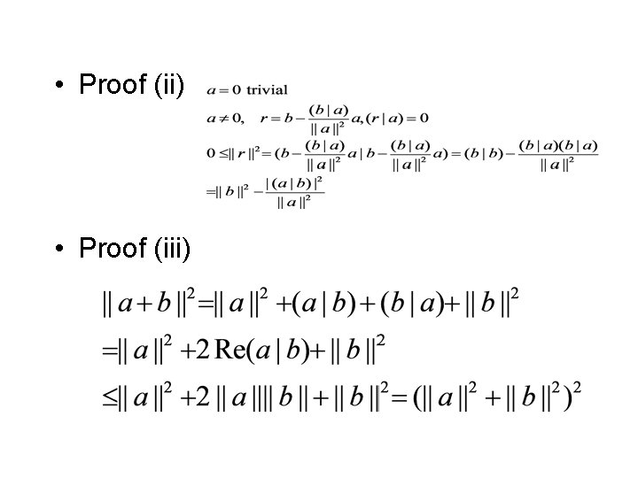
8. 2. Inner product spaces • • Definition: An inner product space (V, ( | )) F⊂R -> Euclidean space F⊂C -> Unitary space. Theorem 1. V, ( | ). Inner product space. 1. 2. 3. 4. ||ca||=|c|||a|| > 0 for a 0. |(a|b)| ||a||||b|| (Cauchy-Schwarz) ||a+b|| ||a||+||b||

• Proof (ii) • Proof (iii)

• In fact many inequalities follows from Cauchy-Schwarz inequality. • The triangle inequality also follows. • See Example 7. • Example 7 (d) is useful in defining Hilbert spaces. Similar inequalities are used much in analysis, PDE, and so on. • Note Example 7, no computations are involved in proving these.

• On inner product spaces one can use the inner product to simplify many things occurring in vector spaces. – Basis -> orthogonal basis. – Projections -> orthogonal projections – Complement -> orthogonal complement. – Linear functions have adjoints – Linear functionals become vector – Operators -> orthogonal operators and self adjoint operators (we restrict to )

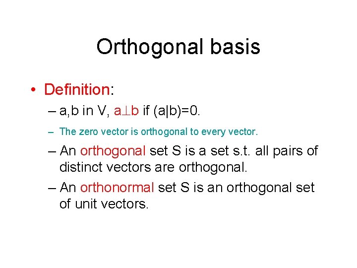
Orthogonal basis • Definition: – a, b in V, a b if (a|b)=0. – The zero vector is orthogonal to every vector. – An orthogonal set S is a set s. t. all pairs of distinct vectors are orthogonal. – An orthonormal set S is an orthogonal set of unit vectors.

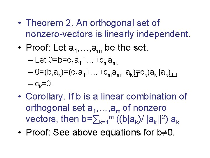
• Theorem 2. An orthogonal set of nonzero-vectors is linearly independent. • Proof: Let a 1, …, am be the set. – Let 0=b=c 1 a 1+…+cmam. – 0=(b, ak)=(c 1 a 1+…+cmam, ak� )=ck(ak |ak� )� – ck=0. • Corollary. If b is a linear combination of orthogonal set a 1, …, am of nonzero vectors, then b=∑k=1 m ((b|ak)/||ak||2) ak • Proof: See above equations for b 0.

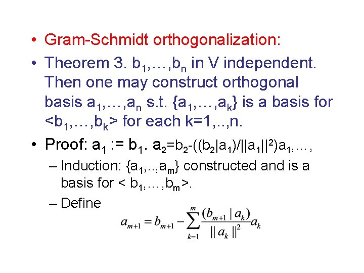
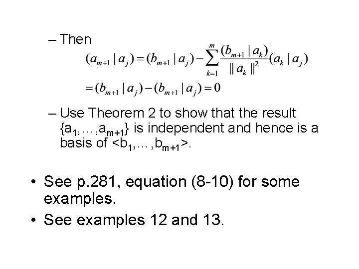
• Gram-Schmidt orthogonalization: • Theorem 3. b 1, …, bn in V independent. Then one may construct orthogonal basis a 1, …, an s. t. {a 1, …, ak} is a basis for <b 1, …, bk> for each k=1, . . , n. • Proof: a 1 : = b 1. a 2=b 2 -((b 2|a 1)/||a 1||2)a 1, …, – Induction: {a 1, . . , am} constructed and is a basis for < b 1, …, bm>. – Define

– Then – Use Theorem 2 to show that the result {a 1, …, am+1} is independent and hence is a basis of <b 1, …, bm+1>. • See p. 281, equation (8 -10) for some examples. • See examples 12 and 13.

Best approximation, Orthogonal complement, Orthogonal projections • This is often used in applied mathematics needing approximations in many cases. • Definition: W a subspace of V. b in W. Then the best approximation of b by a vector in W is a in W s. t. ||b-a|| ||b-c|| for all c in W. • Existence and Uniqueness. (finitedimensional case)

Theorem 4: W a subspace of V. b in V. • • (i). a is a best appr to b <-> b-a c for all c in W. (ii). A best appr is unique (if it exists) (iii). W finite dimensional. {a 1, . . , ak} any orthonormal basis. is the best approx. to b by vectors in W.

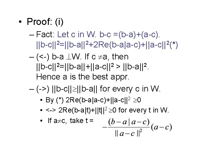
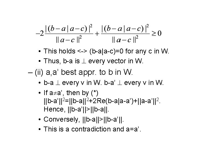
• Proof: (i) – Fact: Let c in W. b-c =(b-a)+(a-c). ||b-c||2=||b-a||2+2 Re(b-a|a-c)+||a-c||2(*) – (<-) b-a W. If c a, then ||b-c||2=||b-a||+||a-c||2 > ||b-a||2. Hence a is the best appr. – (->) ||b-c|| ||b-a|| for every c in W. • By (*) 2 Re(b-a|a-c)+||a-c||2 0 • <-> 2 Re(b-a|t)+||t||2 0 for every t in W. • If a c, take t =

• This holds <-> (b-a|a-c)=0 for any c in W. • Thus, b-a is every vector in W. – (ii) a, a’ best appr. to b in W. • b-a every v in W. b-a’ every v in W. • If a a’, then by (*) ||b-a’||2=||b-a||2+2 Re(b-a|a-a’)+||a-a’||2. Hence, ||b-a’||>||b-a||. • Conversely, ||b-a||>||b-a’||. • This is a contradiction and a=a’.

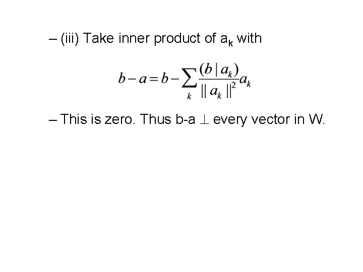
– (iii) Take inner product of ak with – This is zero. Thus b-a every vector in W.

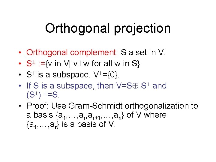
Orthogonal projection • • Orthogonal complement. S a set in V. S : ={v in V| v w for all w in S}. S is a subspace. V ={0}. If S is a subspace, then V=S S and (S ) =S. • Proof: Use Gram-Schmidt orthogonalization to a basis {a 1, …, ar+1, …, an} of V where {a 1, …, ar} is a basis of V.

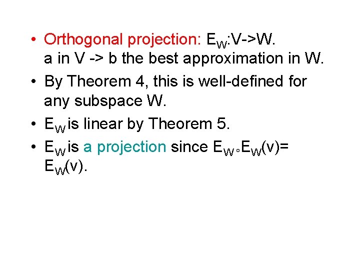
• Orthogonal projection: EW: V->W. a in V -> b the best approximation in W. • By Theorem 4, this is well-defined for any subspace W. • EW is linear by Theorem 5. • EW is a projection since EW EW(v)= EW(v).

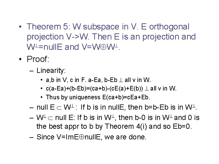
• Theorem 5: W subspace in V. E orthogonal projection V->W. Then E is an projection and W =null. E and V=W W. • Proof: – Linearity: • a, b in V, c in F. a-Ea, b-Eb all v in W. • c(a-Ea)+(b-Eb)=(ca+b)-(c. E(a)+E(b)) all v in W. • Thus by uniqueness E(ca+b)=c. Ea+Eb. – null E W : If b is in null. E, then b=b-Eb is in W. – W null E: If b is in W , then b-0 is in W and 0 is the best appr to b by Theorem 4(i) and so Eb=0. – Since V=Im. E null. E, we are done.

• Corollary: b-> b-Ewb is an orthogonal projection to W. I-Ew is an idempotent linear transformation; i. e. , projection. • Proof: b-> b-Ewb is in W by Theorem 4 (i). – Let c be in W. b-c=Eb+(b-Eb-c). – Eb in W, (b-Eb-c) in W. – ||b-c||2=||Eb||2+||b-Eb-c||2 ||b-(b-Eb)||2 and > if c b-Eb. – Thus, b-Eb is the best appr to b in W.

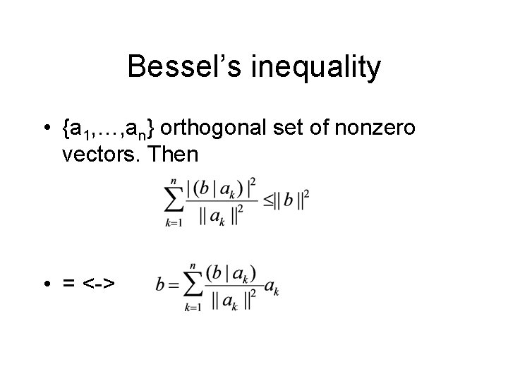
Bessel’s inequality • {a 1, …, an} orthogonal set of nonzero vectors. Then • = <->