Equity Instruments Part I Discounted Cash Flow Valuation

Equity Instruments: Part I Discounted Cash Flow Valuation B 40. 3331 Aswath Damodaran 1

Discounted Cashflow Valuation: Basis for Approach where CFt is the expected cash flow in period t, r is the discount rate appropriate given the riskiness of the cash flow and n is the life of the asset. Proposition 1: For an asset to have value, the expected cash flows have to be positive some time over the life of the asset. Proposition 2: Assets that generate cash flows early in their life will be worth more than assets that generate cash flows later; the latter may however have greater growth and higher cash flows to compensate. 2

DCF Choices: Equity Valuation versus Firm Valuation: Value the entire business Equity valuation: Value just the equity claim in the business 3

Equity Valuation 4

Firm Valuation 5

Firm Value and Equity Value A. B. C. D. A. B. C. To get from firm value to equity value, which of the following would you need to do? Subtract out the value of long term debt Subtract out the value of all debt Subtract the value of any debt that was included in the cost of capital calculation Subtract out the value of all liabilities in the firm Doing so, will give you a value for the equity which is greater than the value you would have got in an equity valuation lesser than the value you would have got in an equity valuation equal to the value you would have got in an equity valuation 6

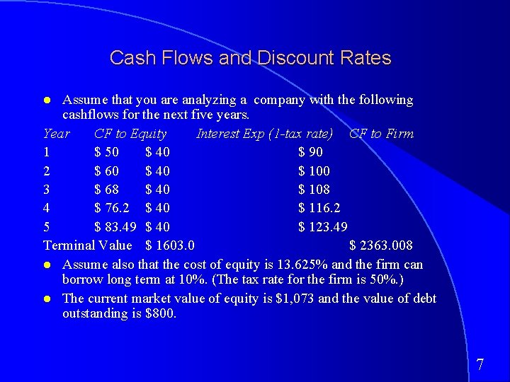
Cash Flows and Discount Rates Assume that you are analyzing a company with the following cashflows for the next five years. Year CF to Equity Interest Exp (1 -tax rate) CF to Firm 1 $ 50 $ 40 $ 90 2 $ 60 $ 40 $ 100 3 $ 68 $ 40 $ 108 4 $ 76. 2 $ 40 $ 116. 2 5 $ 83. 49 $ 40 $ 123. 49 Terminal Value $ 1603. 0 $ 2363. 008 Assume also that the cost of equity is 13. 625% and the firm can borrow long term at 10%. (The tax rate for the firm is 50%. ) The current market value of equity is $1, 073 and the value of debt outstanding is $800. 7

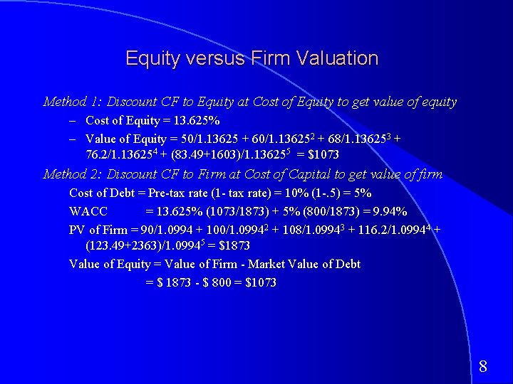
Equity versus Firm Valuation Method 1: Discount CF to Equity at Cost of Equity to get value of equity – Cost of Equity = 13. 625% – Value of Equity = 50/1. 13625 + 60/1. 136252 + 68/1. 136253 + 76. 2/1. 136254 + (83. 49+1603)/1. 136255 = $1073 Method 2: Discount CF to Firm at Cost of Capital to get value of firm Cost of Debt = Pre-tax rate (1 - tax rate) = 10% (1 -. 5) = 5% WACC = 13. 625% (1073/1873) + 5% (800/1873) = 9. 94% PV of Firm = 90/1. 0994 + 100/1. 09942 + 108/1. 09943 + 116. 2/1. 09944 + (123. 49+2363)/1. 09945 = $1873 Value of Equity = Value of Firm - Market Value of Debt = $ 1873 - $ 800 = $1073 8

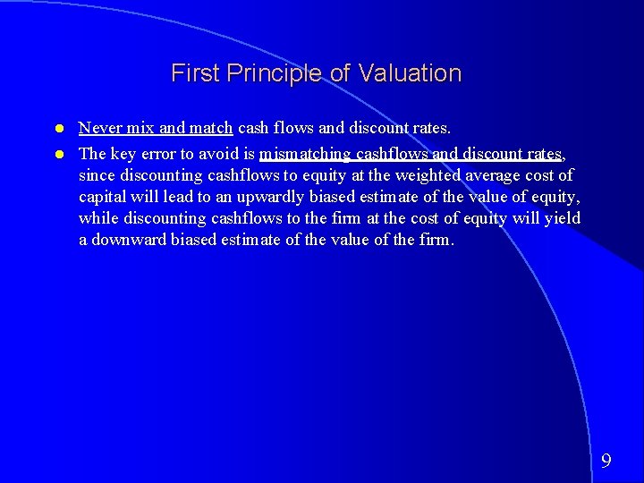
First Principle of Valuation Never mix and match cash flows and discount rates. The key error to avoid is mismatching cashflows and discount rates, since discounting cashflows to equity at the weighted average cost of capital will lead to an upwardly biased estimate of the value of equity, while discounting cashflows to the firm at the cost of equity will yield a downward biased estimate of the value of the firm. 9

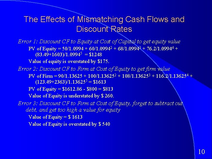
The Effects of Mismatching Cash Flows and Discount Rates Error 1: Discount CF to Equity at Cost of Capital to get equity value PV of Equity = 50/1. 0994 + 60/1. 09942 + 68/1. 09943 + 76. 2/1. 09944 + (83. 49+1603)/1. 09945 = $1248 Value of equity is overstated by $175. Error 2: Discount CF to Firm at Cost of Equity to get firm value PV of Firm = 90/1. 13625 + 100/1. 136252 + 108/1. 136253 + 116. 2/1. 136254 + (123. 49+2363)/1. 136255 = $1613 PV of Equity = $1612. 86 - $800 = $813 Value of Equity is understated by $ 260. Error 3: Discount CF to Firm at Cost of Equity, forget to subtract out debt, and get too high a value for equity Value of Equity = $ 1613 Value of Equity is overstated by $ 540 10

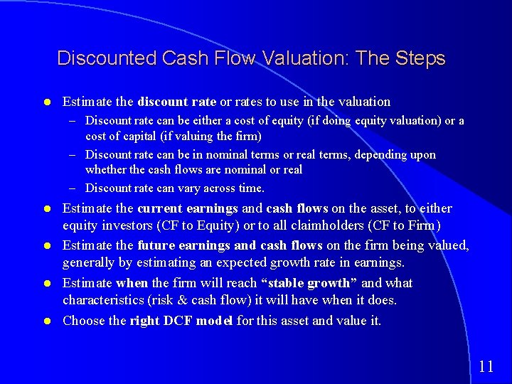
Discounted Cash Flow Valuation: The Steps Estimate the discount rate or rates to use in the valuation – Discount rate can be either a cost of equity (if doing equity valuation) or a cost of capital (if valuing the firm) – Discount rate can be in nominal terms or real terms, depending upon whether the cash flows are nominal or real – Discount rate can vary across time. Estimate the current earnings and cash flows on the asset, to either equity investors (CF to Equity) or to all claimholders (CF to Firm) Estimate the future earnings and cash flows on the firm being valued, generally by estimating an expected growth rate in earnings. Estimate when the firm will reach “stable growth” and what characteristics (risk & cash flow) it will have when it does. Choose the right DCF model for this asset and value it. 11

Generic DCF Valuation Model 12

13

14

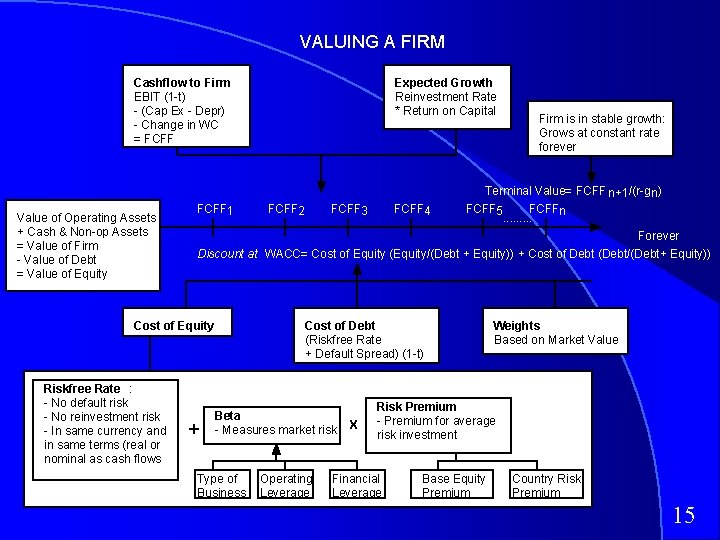
VALUING A FIRM Cashflow to Firm EBIT (1 -t) - (Cap Ex - Depr) - Change in WC = FCFF Value of Operating Assets + Cash & Non-op Assets = Value of Firm - Value of Debt = Value of Equity Firm is in stable growth: Grows at constant rate forever Terminal Value= FCFF n+1 /(r-gn) FCFF 1 FCFF 2 FCFF 3 FCFF 4 FCFF 5 FCFFn. . Forever Discount at WACC= Cost of Equity (Equity/(Debt + Equity)) + Cost of Debt (Debt/(Debt+ Equity)) Cost of Equity Riskfree Rate : - No default risk - No reinvestment risk - In same currency and in same terms (real or nominal as cash flows Expected Growth Reinvestment Rate * Return on Capital + Cost of Debt (Riskfree Rate + Default Spread) (1 -t) Beta - Measures market risk Type of Business Operating Leverage X Weights Based on Market Value Risk Premium - Premium for average risk investment Financial Leverage Base Equity Premium Country Risk Premium 15

Discounted Cash Flow Valuation: The Inputs Aswath Damodaran 16

I. Estimating Discount Rates DCF Valuation 17

Estimating Inputs: Discount Rates Critical ingredient in discounted cashflow valuation. Errors in estimating the discount rate or mismatching cashflows and discount rates can lead to serious errors in valuation. At an intuitive level, the discount rate used should be consistent with both the riskiness and the type of cashflow being discounted. – Equity versus Firm: If the cash flows being discounted are cash flows to equity, the appropriate discount rate is a cost of equity. If the cash flows are cash flows to the firm, the appropriate discount rate is the cost of capital. – Currency: The currency in which the cash flows are estimated should also be the currency in which the discount rate is estimated. – Nominal versus Real: If the cash flows being discounted are nominal cash flows (i. e. , reflect expected inflation), the discount rate should be nominal 18

Cost of Equity The cost of equity should be higher for riskier investments and lower for safer investments While risk is usually defined in terms of the variance of actual returns around an expected return, risk and return models in finance assume that the risk that should be rewarded (and thus built into the discount rate) in valuation should be the risk perceived by the marginal investor in the investment Most risk and return models in finance also assume that the marginal investor is well diversified, and that the only risk that he or she perceives in an investment is risk that cannot be diversified away (I. e, market or non-diversifiable risk) 19

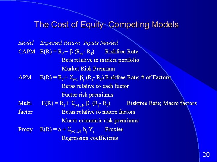
The Cost of Equity: Competing Models Model Expected Return Inputs Needed CAPM E(R) = Rf + (Rm- Rf) Riskfree Rate Beta relative to market portfolio Market Risk Premium APM E(R) = Rf + j=1 j (Rj- Rf) Riskfree Rate; # of Factors; Betas relative to each factor Factor risk premiums Multi E(R) = Rf + j=1, , N j (Rj- Rf) Riskfree Rate; Macro factors factor Betas relative to macro factors Macro economic risk premiums Proxy E(R) = a + j=1. . N bj Yj Proxies Regression coefficients 20

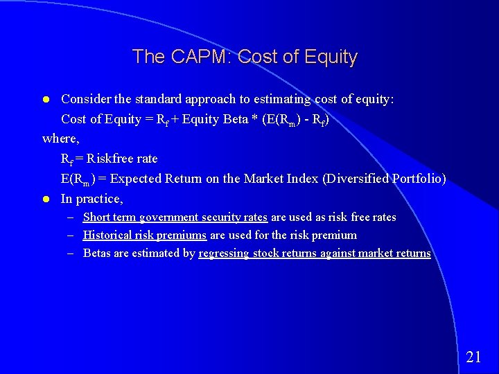
The CAPM: Cost of Equity Consider the standard approach to estimating cost of equity: Cost of Equity = Rf + Equity Beta * (E(Rm) - Rf) where, Rf = Riskfree rate E(Rm) = Expected Return on the Market Index (Diversified Portfolio) In practice, – Short term government security rates are used as risk free rates – Historical risk premiums are used for the risk premium – Betas are estimated by regressing stock returns against market returns 21

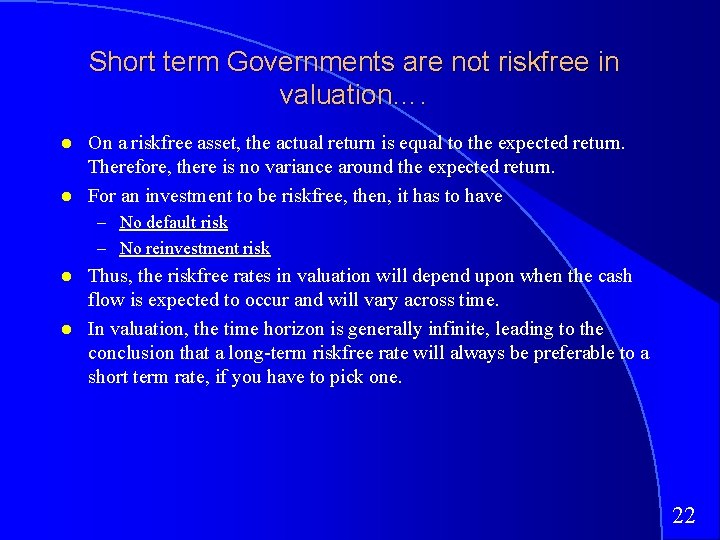
Short term Governments are not riskfree in valuation…. On a riskfree asset, the actual return is equal to the expected return. Therefore, there is no variance around the expected return. For an investment to be riskfree, then, it has to have – No default risk – No reinvestment risk Thus, the riskfree rates in valuation will depend upon when the cash flow is expected to occur and will vary across time. In valuation, the time horizon is generally infinite, leading to the conclusion that a long-term riskfree rate will always be preferable to a short term rate, if you have to pick one. 22

Riskfree Rates in 2004 23

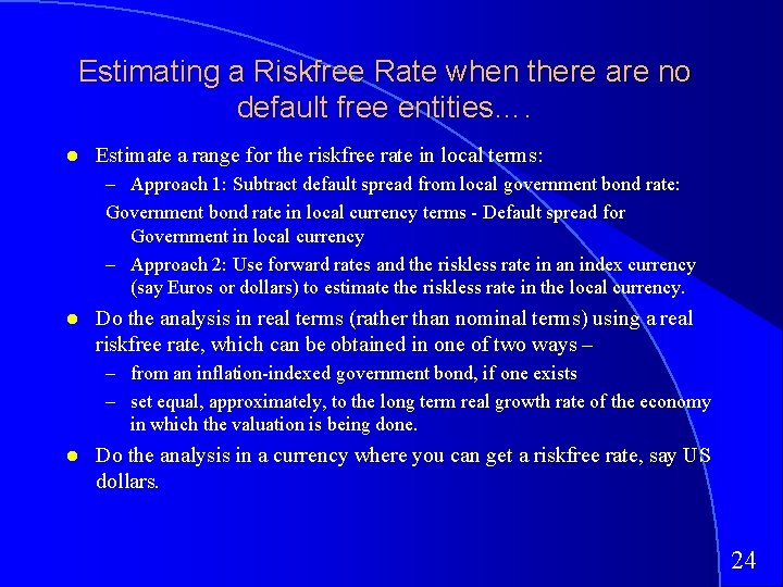
Estimating a Riskfree Rate when there are no default free entities…. Estimate a range for the riskfree rate in local terms: – Approach 1: Subtract default spread from local government bond rate: Government bond rate in local currency terms - Default spread for Government in local currency – Approach 2: Use forward rates and the riskless rate in an index currency (say Euros or dollars) to estimate the riskless rate in the local currency. Do the analysis in real terms (rather than nominal terms) using a real riskfree rate, which can be obtained in one of two ways – – from an inflation-indexed government bond, if one exists – set equal, approximately, to the long term real growth rate of the economy in which the valuation is being done. Do the analysis in a currency where you can get a riskfree rate, say US dollars. 24

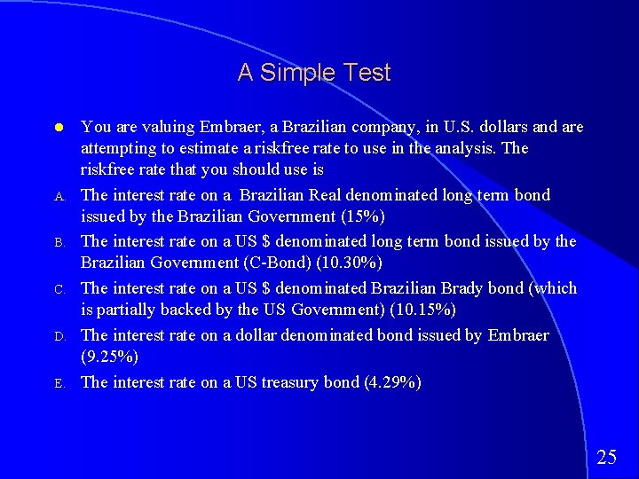
A Simple Test A. B. C. D. E. You are valuing Embraer, a Brazilian company, in U. S. dollars and are attempting to estimate a riskfree rate to use in the analysis. The riskfree rate that you should use is The interest rate on a Brazilian Real denominated long term bond issued by the Brazilian Government (15%) The interest rate on a US $ denominated long term bond issued by the Brazilian Government (C-Bond) (10. 30%) The interest rate on a US $ denominated Brazilian Brady bond (which is partially backed by the US Government) (10. 15%) The interest rate on a dollar denominated bond issued by Embraer (9. 25%) The interest rate on a US treasury bond (4. 29%) 25

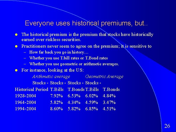
Everyone uses historical premiums, but. . The historical premium is the premium that stocks have historically earned over riskless securities. Practitioners never seem to agree on the premium; it is sensitive to – How far back you go in history… – Whether you use T. bill rates or T. Bond rates – Whether you use geometric or arithmetic averages. For instance, looking at the US: Arithmetic average Geometric Average Stocks - Stocks Historical Period T. Bills T. Bonds 1928 -2004 7. 92% 6. 53% 6. 02% 4. 84% 1964 -2004 5. 82% 4. 34% 4. 59% 3. 47% 1994 -2004 8. 60% 5. 82% 6. 85% 4. 51% 26

If you choose to use historical premiums…. Go back as far as you can. A risk premium comes with a standard error. Given the annual standard deviation in stock prices is about 25%, the standard error in a historical premium estimated over 25 years is roughly: Standard Error in Premium = 25%/√ 25 = 25%/5 = 5% Be consistent in your use of the riskfree rate. Since we argued for long term bond rates, the premium should be the one over T. Bonds Use the geometric risk premium. It is closer to how investors think about risk premiums over long periods. 27

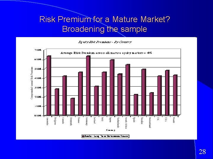
Risk Premium for a Mature Market? Broadening the sample 28

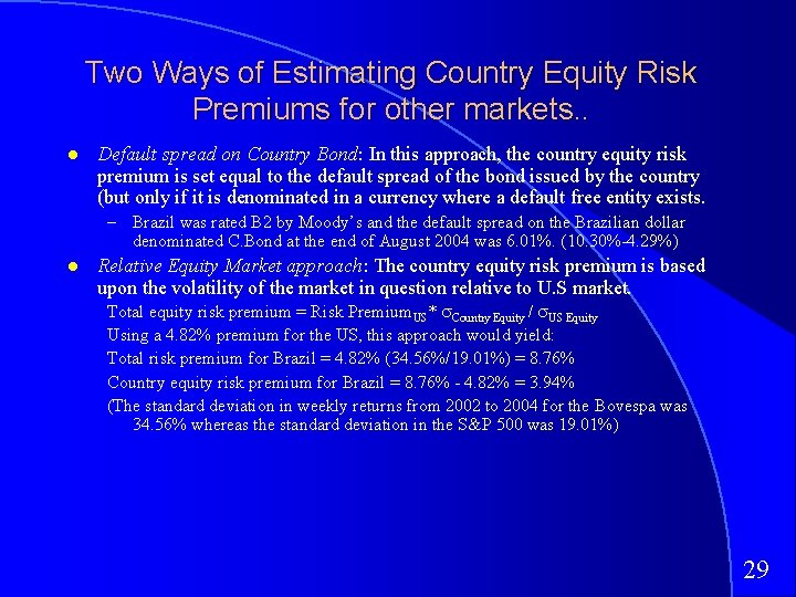
Two Ways of Estimating Country Equity Risk Premiums for other markets. . Default spread on Country Bond: In this approach, the country equity risk premium is set equal to the default spread of the bond issued by the country (but only if it is denominated in a currency where a default free entity exists. – Brazil was rated B 2 by Moody’s and the default spread on the Brazilian dollar denominated C. Bond at the end of August 2004 was 6. 01%. (10. 30%-4. 29%) Relative Equity Market approach: The country equity risk premium is based upon the volatility of the market in question relative to U. S market. Total equity risk premium = Risk Premium. US* Country Equity / US Equity Using a 4. 82% premium for the US, this approach would yield: Total risk premium for Brazil = 4. 82% (34. 56%/19. 01%) = 8. 76% Country equity risk premium for Brazil = 8. 76% - 4. 82% = 3. 94% (The standard deviation in weekly returns from 2002 to 2004 for the Bovespa was 34. 56% whereas the standard deviation in the S&P 500 was 19. 01%) 29

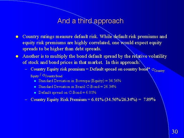
And a third approach Country ratings measure default risk. While default risk premiums and equity risk premiums are highly correlated, one would expect equity spreads to be higher than debt spreads. Another is to multiply the bond default spread by the relative volatility of stock and bond prices in that market. In this approach: – Country Equity risk premium = Default spread on country bond* Country Equity / Country Bond Standard Deviation in Bovespa (Equity) = 34. 56% Standard Deviation in Brazil C-Bond = 26. 34% Default spread on C-Bond = 6. 01% – Country Equity Risk Premium = 6. 01% (34. 56%/26. 34%) = 7. 89% 30

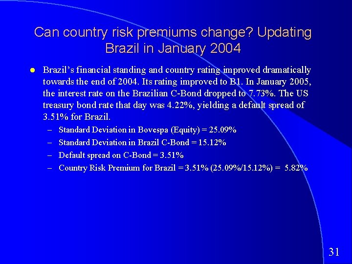
Can country risk premiums change? Updating Brazil in January 2004 Brazil’s financial standing and country rating improved dramatically towards the end of 2004. Its rating improved to B 1. In January 2005, the interest rate on the Brazilian C-Bond dropped to 7. 73%. The US treasury bond rate that day was 4. 22%, yielding a default spread of 3. 51% for Brazil. – – Standard Deviation in Bovespa (Equity) = 25. 09% Standard Deviation in Brazil C-Bond = 15. 12% Default spread on C-Bond = 3. 51% Country Risk Premium for Brazil = 3. 51% (25. 09%/15. 12%) = 5. 82% 31

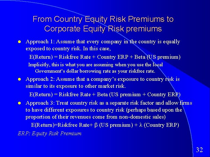
From Country Equity Risk Premiums to Corporate Equity Risk premiums Approach 1: Assume that every company in the country is equally exposed to country risk. In this case, E(Return) = Riskfree Rate + Country ERP + Beta (US premium) Implicitly, this is what you are assuming when you use the local Government’s dollar borrowing rate as your riskfree rate. Approach 2: Assume that a company’s exposure to country risk is similar to its exposure to other market risk. E(Return) = Riskfree Rate + Beta (US premium + Country ERP) Approach 3: Treat country risk as a separate risk factor and allow firms to have different exposures to country risk (perhaps based upon the proportion of their revenues come from non-domestic sales) E(Return)=Riskfree Rate+ (US premium) + (Country ERP) ERP: Equity Risk Premium 32

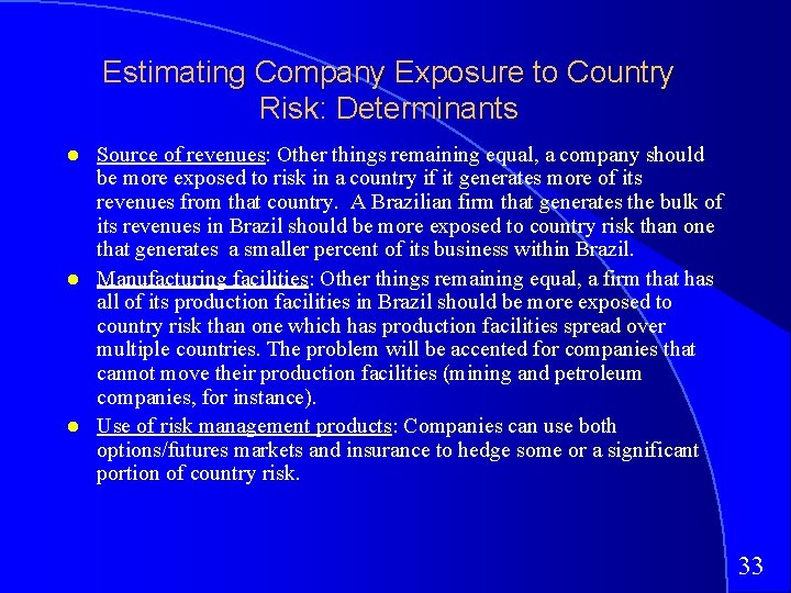
Estimating Company Exposure to Country Risk: Determinants Source of revenues: Other things remaining equal, a company should be more exposed to risk in a country if it generates more of its revenues from that country. A Brazilian firm that generates the bulk of its revenues in Brazil should be more exposed to country risk than one that generates a smaller percent of its business within Brazil. Manufacturing facilities: Other things remaining equal, a firm that has all of its production facilities in Brazil should be more exposed to country risk than one which has production facilities spread over multiple countries. The problem will be accented for companies that cannot move their production facilities (mining and petroleum companies, for instance). Use of risk management products: Companies can use both options/futures markets and insurance to hedge some or a significant portion of country risk. 33

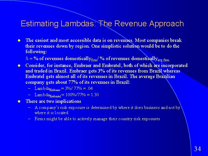
Estimating Lambdas: The Revenue Approach The easiest and most accessible data is on revenues. Most companies break their revenues down by region. One simplistic solution would be to do the following: = % of revenues domesticallyfirm/ % of revenues domesticallyavg firm Consider, for instance, Embraer and Embratel, both of which are incorporated and traded in Brazil. Embraer gets 3% of its revenues from Brazil whereas Embratel gets almost all of its revenues in Brazil. The average Brazilian company gets about 77% of its revenues in Brazil: – Lambda. Embraer = 3%/ 77% =. 04 – Lambda. Embratel = 100%/77% = 1. 30 There are two implications – A company’s risk exposure is determined by where it does business and not by where it is located – Firms might be able to actively manage their country risk exposures 34

Estimating Lambdas: Earnings Approach 35

Estimating Lambdas: Stock Returns versus CBond Returns Return. Embraer = 0. 0195 + 0. 2681 Return. C Bond Return. Embratel = -0. 0308 + 2. 0030 Return. C Bond 36

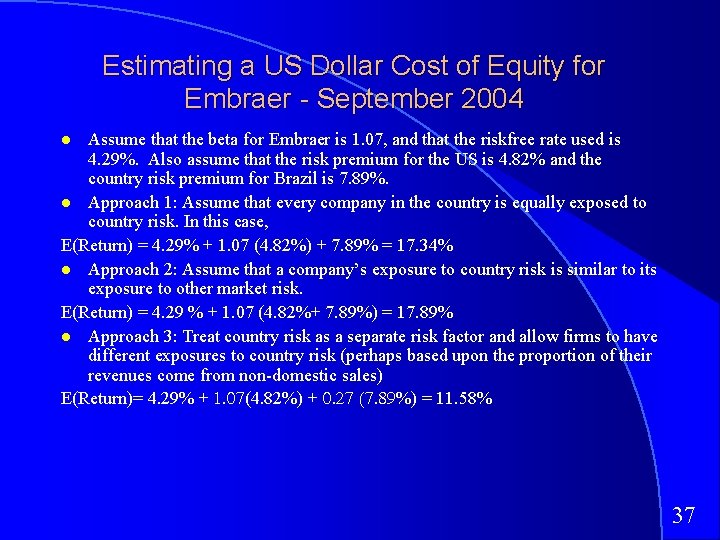
Estimating a US Dollar Cost of Equity for Embraer - September 2004 Assume that the beta for Embraer is 1. 07, and that the riskfree rate used is 4. 29%. Also assume that the risk premium for the US is 4. 82% and the country risk premium for Brazil is 7. 89%. Approach 1: Assume that every company in the country is equally exposed to country risk. In this case, E(Return) = 4. 29% + 1. 07 (4. 82%) + 7. 89% = 17. 34% Approach 2: Assume that a company’s exposure to country risk is similar to its exposure to other market risk. E(Return) = 4. 29 % + 1. 07 (4. 82%+ 7. 89%) = 17. 89% Approach 3: Treat country risk as a separate risk factor and allow firms to have different exposures to country risk (perhaps based upon the proportion of their revenues come from non-domestic sales) E(Return)= 4. 29% + 1 7(4. 82%) + 27 (7 %) = 11. 58% 37

Valuing Emerging Market Companies with significant exposure in developed markets A. B. § The conventional practice in investment banking is to add the country equity risk premium on to the cost of equity for every emerging market company, notwithstanding its exposure to emerging market risk. Thus, Embraer would have been valued with a cost of equity of 17. 34% even though it gets only 3% of its revenues in Brazil. As an investor, which of the following consequences do you see from this approach? Emerging market companies with substantial exposure in developed markets will be significantly over valued by equity research analysts. Emerging market companies with substantial exposure in developed markets will be significantly under valued by equity research analysts. Can you construct an investment strategy to take advantage of the misvaluation? 38

Implied Equity Premiums If we assume that stocks are correctly priced in the aggregate and we can estimate the expected cashflows from buying stocks, we can estimate the expected rate of return on stocks by computing an internal rate of return. Subtracting out the riskfree rate should yield an implied equity risk premium. This implied equity premium is a forward looking number and can be updated as often as you want (every minute of every day, if you are so inclined). 39

Implied Equity Premiums We can use the information in stock prices to back out how risk averse the market is and how much of a risk premium it is demanding. If you pay the current level of the index, you can expect to make a return of 7. 87% on stocks (which is obtained by solving for r in the following equation) Implied Equity risk premium = Expected return on stocks - Treasury bond rate = 7. 87% 4. 22% = 3. 65% 40

Implied Risk Premium Dynamics Assume that the index jumps 10% on January 2 and that nothing else changes. What will happen to the implied equity risk premium? Implied equity risk premium will increase Implied equity risk premium will decrease Assume that the earnings jump 10% on January 2 and that nothing else changes. What will happen to the implied equity risk premium? Implied equity risk premium will increase Implied equity risk premium will decrease Assume that the riskfree rate increases to 5% on January 2 and that nothing else changes. What will happen to the implied equity risk premium? Implied equity risk premium will increase Implied equity risk premium will decrease 41

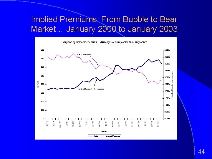
Implied Premiums in the US 42

Implied Premium versus Risk. Free Rate 43

Implied Premiums: From Bubble to Bear Market… January 2000 to January 2003 44

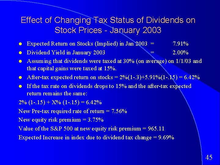
Effect of Changing Tax Status of Dividends on Stock Prices - January 2003 Expected Return on Stocks (Implied) in Jan 2003 = 7. 91% Dividend Yield in January 2003 = 2. 00% Assuming that dividends were taxed at 30% (on average) on 1/1/03 and that capital gains were taxed at 15%. After-tax expected return on stocks = 2%(1 -. 3)+5. 91%(1 -. 15) = 6. 42% If the tax rate on dividends drops to 15% and the after-tax expected return remains the same: 2% (1 -. 15) + X% (1 -. 15) = 6. 42% New Pre-tax required rate of return = 7. 56% New equity risk premium = 3. 75% Value of the S&P 500 at new equity risk premium = 965. 11 Expected Increase in index due to dividend tax change = 9. 69% 45

Which equity risk premium should you use for the US? Historical Risk Premium: When you use the historical risk premium, you are assuming that premiums will revert back to a historical norm and that the time period that you are using is the right norm. You are also more likely to find stocks to be overvalued than undervalued (Why? ) Current Implied Equity Risk premium: You are assuming that the market is correct in the aggregate but makes mistakes on individual stocks. If you are required to be market neutral, this is the premium you should use. (What types of valuations require market neutrality? ) Average Implied Equity Risk premium: The average implied equity risk premium between 1960 -2003 in the United States is about 4%. You are assuming that the market is correct on average but not necessarily at a point in time. 46

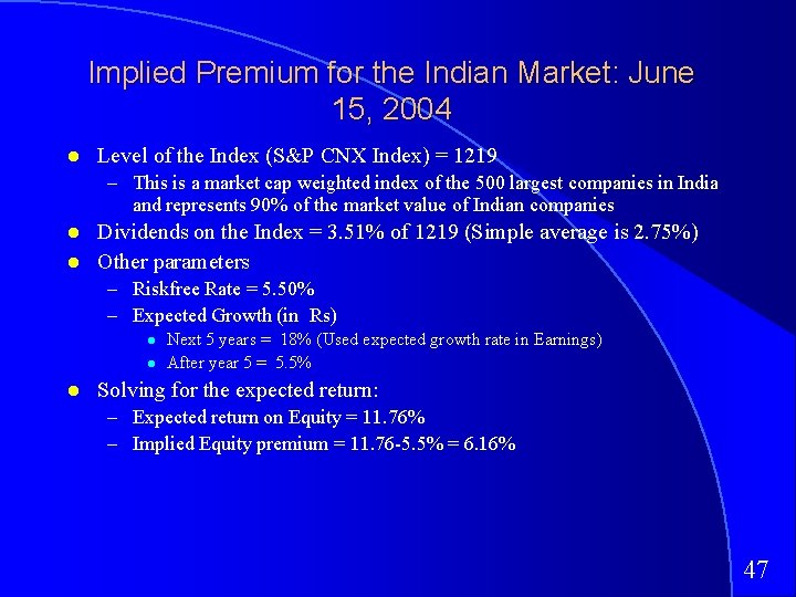
Implied Premium for the Indian Market: June 15, 2004 Level of the Index (S&P CNX Index) = 1219 – This is a market cap weighted index of the 500 largest companies in India and represents 90% of the market value of Indian companies Dividends on the Index = 3. 51% of 1219 (Simple average is 2. 75%) Other parameters – Riskfree Rate = 5. 50% – Expected Growth (in Rs) Next 5 years = 18% (Used expected growth rate in Earnings) After year 5 = 5. 5% Solving for the expected return: – Expected return on Equity = 11. 76% – Implied Equity premium = 11. 76 -5. 5% = 6. 16% 47

Implied Equity Risk Premium for Germany: September 23, 2004 We can use the information in stock prices to back out how risk averse the market is and how much of a risk premium it is demanding. If you pay the current level of the index, you can expect to make a return of 7. 78% on stocks (which is obtained by solving for r in the following equation) Implied Equity risk premium = Expected return on stocks - Treasury bond rate = 7. 78% - 3. 95% = 3. 83% 48

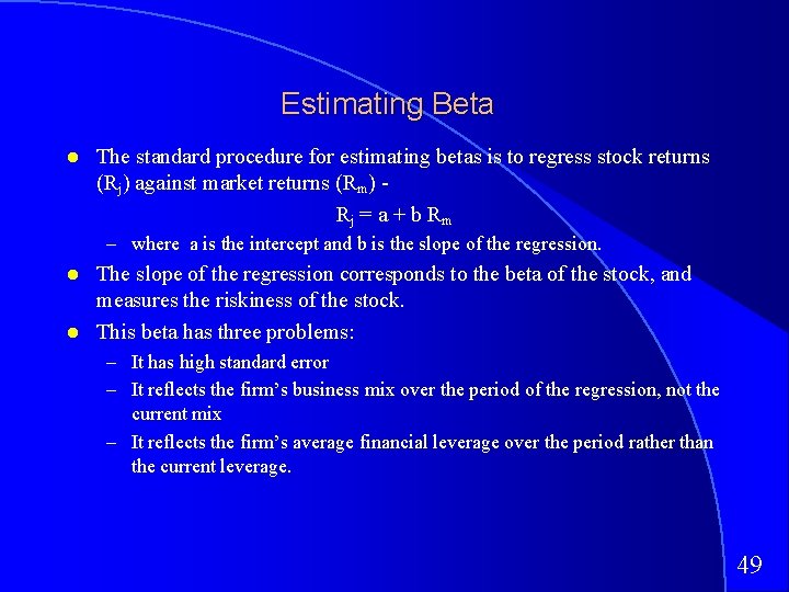
Estimating Beta The standard procedure for estimating betas is to regress stock returns (Rj) against market returns (Rm) Rj = a + b Rm – where a is the intercept and b is the slope of the regression. The slope of the regression corresponds to the beta of the stock, and measures the riskiness of the stock. This beta has three problems: – It has high standard error – It reflects the firm’s business mix over the period of the regression, not the current mix – It reflects the firm’s average financial leverage over the period rather than the current leverage. 49

Beta Estimation: The Noise Problem 50

Beta Estimation: The Index Effect 51

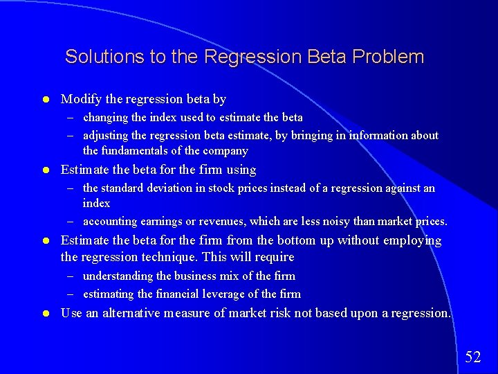
Solutions to the Regression Beta Problem Modify the regression beta by – changing the index used to estimate the beta – adjusting the regression beta estimate, by bringing in information about the fundamentals of the company Estimate the beta for the firm using – the standard deviation in stock prices instead of a regression against an index – accounting earnings or revenues, which are less noisy than market prices. Estimate the beta for the firm from the bottom up without employing the regression technique. This will require – understanding the business mix of the firm – estimating the financial leverage of the firm Use an alternative measure of market risk not based upon a regression. 52

The Index Game… 53

Determinants of Betas 54

In a perfect world… we would estimate the beta of a firm by doing the following 55

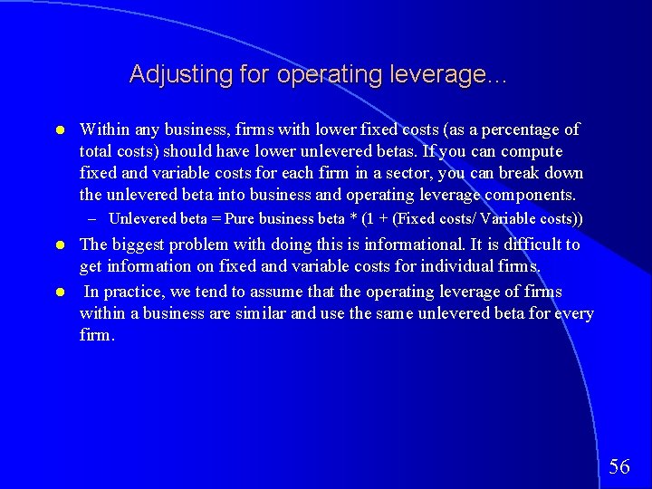
Adjusting for operating leverage… Within any business, firms with lower fixed costs (as a percentage of total costs) should have lower unlevered betas. If you can compute fixed and variable costs for each firm in a sector, you can break down the unlevered beta into business and operating leverage components. – Unlevered beta = Pure business beta * (1 + (Fixed costs/ Variable costs)) The biggest problem with doing this is informational. It is difficult to get information on fixed and variable costs for individual firms. In practice, we tend to assume that the operating leverage of firms within a business are similar and use the same unlevered beta for every firm. 56

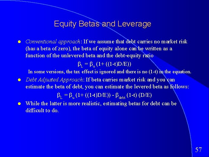
Equity Betas and Leverage Conventional approach: If we assume that debt carries no market risk (has a beta of zero), the beta of equity alone can be written as a function of the unlevered beta and the debt-equity ratio L = u (1+ ((1 -t)D/E)) In some versions, the tax effect is ignored and there is no (1 -t) in the equation. Debt Adjusted Approach: If beta carries market risk and you can estimate the beta of debt, you can estimate the levered beta as follows: L = u (1+ ((1 -t)D/E)) - debt (1 -t) (D/E) While the latter is more realistic, estimating betas for debt can be difficult to do. 57

Bottom-up Betas 58

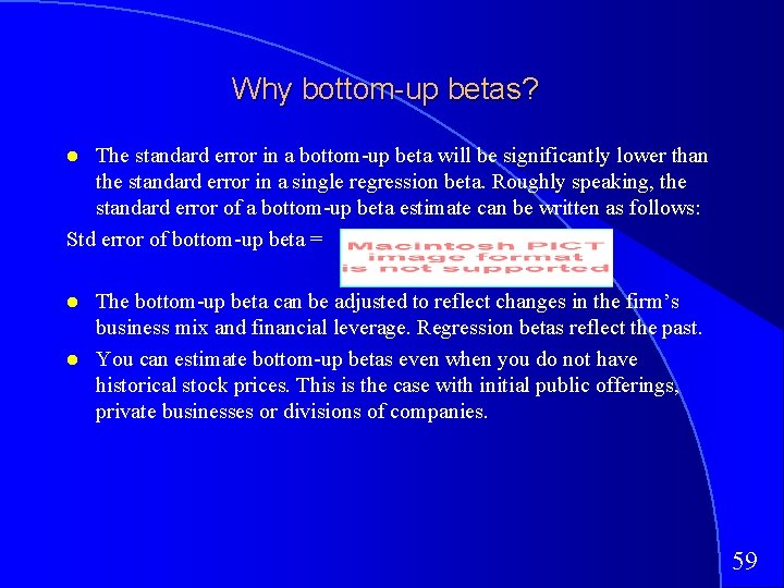
Why bottom-up betas? The standard error in a bottom-up beta will be significantly lower than the standard error in a single regression beta. Roughly speaking, the standard error of a bottom-up beta estimate can be written as follows: Std error of bottom-up beta = The bottom-up beta can be adjusted to reflect changes in the firm’s business mix and financial leverage. Regression betas reflect the past. You can estimate bottom-up betas even when you do not have historical stock prices. This is the case with initial public offerings, private businesses or divisions of companies. 59

Bottom-up Beta: Firm in Multiple Businesses Disney in 2003 Start with the unlevered betas for the businesses Estimate the unlevered beta for Disney’s businesses Estimate a levered beta for Disney Market debt to equity ratio = 37. 46% Marginal tax rate = 37. 60% Levered beta = 1. 1258 ( 1 + (1 -. 376) (. 3746)) = 1. 39 60

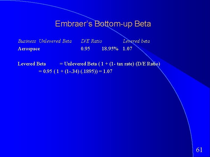
Embraer’s Bottom-up Beta Business Unlevered Beta Aerospace D/E Ratio Levered beta 0. 95 18. 95% 1. 07 Levered Beta = Unlevered Beta ( 1 + (1 - tax rate) (D/E Ratio) = 0. 95 ( 1 + (1 -. 34) (. 1895)) = 1. 07 61

Comparable Firms? Can an unlevered beta estimated using U. S. and European aerospace companies be used to estimate the beta for a Brazilian aerospace company? q Yes q No What concerns would you have in making this assumption? 62

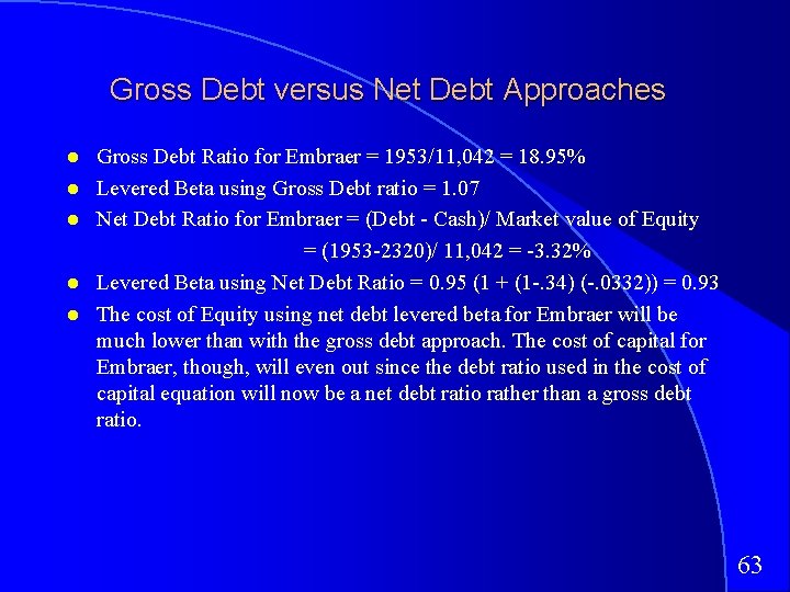
Gross Debt versus Net Debt Approaches Gross Debt Ratio for Embraer = 1953/11, 042 = 18. 95% Levered Beta using Gross Debt ratio = 1. 07 Net Debt Ratio for Embraer = (Debt - Cash)/ Market value of Equity = (1953 -2320)/ 11, 042 = -3. 32% Levered Beta using Net Debt Ratio = 0. 95 (1 + (1 -. 34) (-. 0332)) = 0. 93 The cost of Equity using net debt levered beta for Embraer will be much lower than with the gross debt approach. The cost of capital for Embraer, though, will even out since the debt ratio used in the cost of capital equation will now be a net debt ratio rather than a gross debt ratio. 63

The Cost of Equity: A Recap 64

Estimating the Cost of Debt The cost of debt is the rate at which you can borrow at currently, It will reflect not only your default risk but also the level of interest rates in the market. The two most widely used approaches to estimating cost of debt are: – Looking up the yield to maturity on a straight bond outstanding from the firm. The limitation of this approach is that very few firms have long term straight bonds that are liquid and widely traded – Looking up the rating for the firm and estimating a default spread based upon the rating. While this approach is more robust, different bonds from the same firm can have different ratings. You have to use a median rating for the firm When in trouble (either because you have no ratings or multiple ratings for a firm), estimate a synthetic rating for your firm and the cost of debt based upon that rating. 65

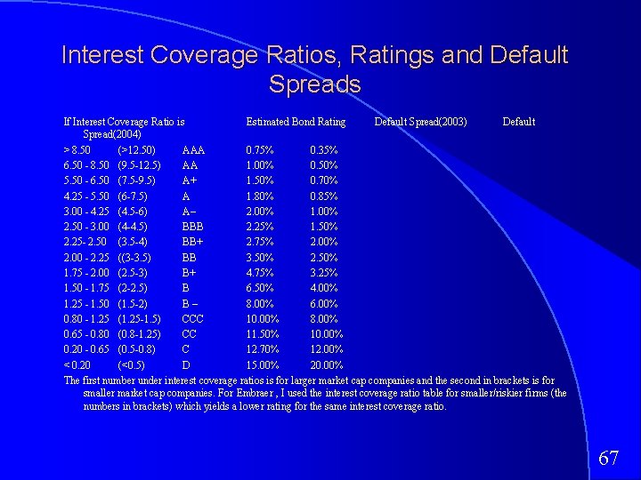
Estimating Synthetic Ratings The rating for a firm can be estimated using the financial characteristics of the firm. In its simplest form, the rating can be estimated from the interest coverage ratio Interest Coverage Ratio = EBIT / Interest Expenses For Embraer’s interest coverage ratio, we used the interest expenses from 2003 and the average EBIT from 2001 to 2003. (The aircraft business was badly affected by 9/11 and its aftermath. In 2002 and 2003, Embraer reported significant drops in operating income) – Interest Coverage Ratio = 462. 1 /129. 70 = 3. 56 66

Interest Coverage Ratios, Ratings and Default Spreads If Interest Coverage Ratio is Estimated Bond Rating Default Spread(2003) Default Spread(2004) > 8. 50 (>12. 50) AAA 0. 75% 0. 35% 6. 50 - 8. 50 (9. 5 -12. 5) AA 1. 00% 0. 50% 5. 50 - 6. 50 (7. 5 -9. 5) A+ 1. 50% 0. 70% 4. 25 - 5. 50 (6 -7. 5) A 1. 80% 0. 85% 3. 00 - 4. 25 (4. 5 -6) A– 2. 00% 1. 00% 2. 50 - 3. 00 (4 -4. 5) BBB 2. 25% 1. 50% 2. 25 - 2. 50 (3. 5 -4) BB+ 2. 75% 2. 00 - 2. 25 ((3 -3. 5) BB 3. 50% 2. 50% 1. 75 - 2. 00 (2. 5 -3) B+ 4. 75% 3. 25% 1. 50 - 1. 75 (2 -2. 5) B 6. 50% 4. 00% 1. 25 - 1. 50 (1. 5 -2) B– 8. 00% 6. 00% 0. 80 - 1. 25 (1. 25 -1. 5) CCC 10. 00% 8. 00% 0. 65 - 0. 80 (0. 8 -1. 25) CC 11. 50% 10. 00% 0. 20 - 0. 65 (0. 5 -0. 8) C 12. 70% 12. 00% < 0. 20 (<0. 5) D 15. 00% 20. 00% The first number under interest coverage ratios is for larger market cap companies and the second in brackets is for smaller market cap companies. For Embraer , I used the interest coverage ratio table for smaller/riskier firms (the numbers in brackets) which yields a lower rating for the same interest coverage ratio. 67

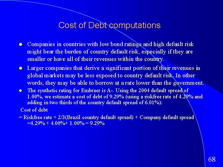
Cost of Debt computations Companies in countries with low bond ratings and high default risk might bear the burden of country default risk, especially if they are smaller or have all of their revenues within the country. Larger companies that derive a significant portion of their revenues in global markets may be less exposed to country default risk. In other words, they may be able to borrow at a rate lower than the government. The synthetic rating for Embraer is A-. Using the 2004 default spread of 1. 00%, we estimate a cost of debt of 9. 29% (using a riskfree rate of 4. 29% and adding in two thirds of the country default spread of 6. 01%): Cost of debt = Riskfree rate + 2/3(Brazil country default spread) + Company default spread =4. 29% + 4. 00%+ 1. 00% = 9. 29% 68

Synthetic Ratings: Some Caveats The relationship between interest coverage ratios and ratings, developed using US companies, tends to travel well, as long as we are analyzing large manufacturing firms in markets with interest rates close to the US interest rate They are more problematic when looking at smaller companies in markets with higher interest rates than the US. 69

Weights for the Cost of Capital Computation The weights used to compute the cost of capital should be the market value weights for debt and equity. There is an element of circularity that is introduced into every valuation by doing this, since the values that we attach to the firm and equity at the end of the analysis are different from the values we gave them at the beginning. As a general rule, the debt that you should subtract from firm value to arrive at the value of equity should be the same debt that you used to compute the cost of capital. 70

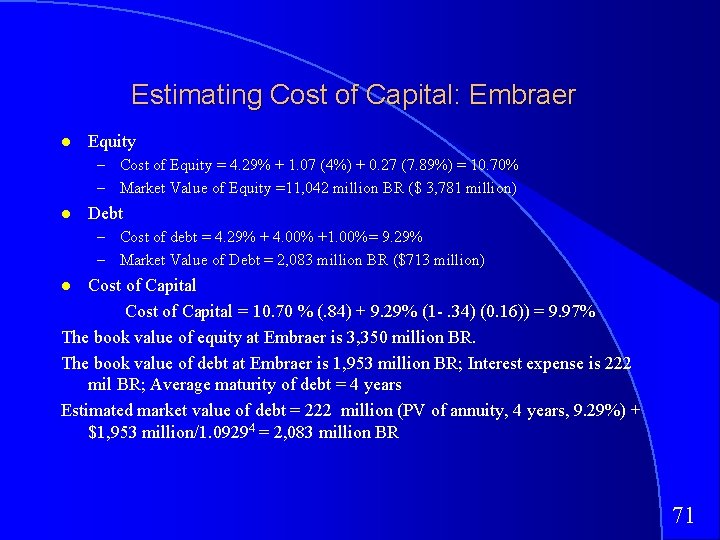
Estimating Cost of Capital: Embraer Equity – Cost of Equity = 4. 29% + 1. 07 (4%) + 0. 27 (7. 89%) = 10. 70% – Market Value of Equity =11, 042 million BR ($ 3, 781 million) Debt – Cost of debt = 4. 29% + 4. 00% +1. 00%= 9. 29% – Market Value of Debt = 2, 083 million BR ($713 million) Cost of Capital = 10. 70 % (. 84) + 9. 29% (1 -. 34) (0. 16)) = 9. 97% The book value of equity at Embraer is 3, 350 million BR. The book value of debt at Embraer is 1, 953 million BR; Interest expense is 222 mil BR; Average maturity of debt = 4 years Estimated market value of debt = 222 million (PV of annuity, 4 years, 9. 29%) + $1, 953 million/1. 09294 = 2, 083 million BR 71

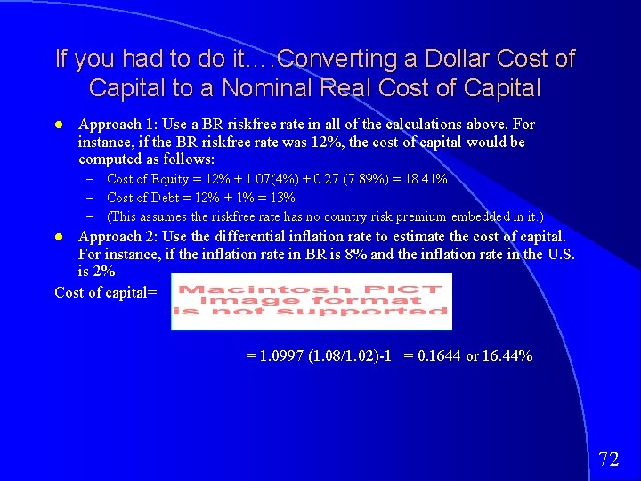
If you had to do it…. Converting a Dollar Cost of Capital to a Nominal Real Cost of Capital Approach 1: Use a BR riskfree rate in all of the calculations above. For instance, if the BR riskfree rate was 12%, the cost of capital would be computed as follows: – Cost of Equity = 12% + 1 7(4%) + 27 (7 %) = 18. 41% – Cost of Debt = 12% + 1% = 13% – (This assumes the riskfree rate has no country risk premium embedded in it. ) Approach 2: Use the differential inflation rate to estimate the cost of capital. For instance, if the inflation rate in BR is 8% and the inflation rate in the U. S. is 2% Cost of capital= = 1. 0997 (1. 08/1. 02)-1 = 0. 1644 or 16. 44% 72

Dealing with Hybrids and Preferred Stock When dealing with hybrids (convertible bonds, for instance), break the security down into debt and equity and allocate the amounts accordingly. Thus, if a firm has $ 125 million in convertible debt outstanding, break the $125 million into straight debt and conversion option components. The conversion option is equity. When dealing with preferred stock, it is better to keep it as a separate component. The cost of preferred stock is the preferred dividend yield. (As a rule of thumb, if the preferred stock is less than 5% of the outstanding market value of the firm, lumping it in with debt will make no significant impact on your valuation). 73

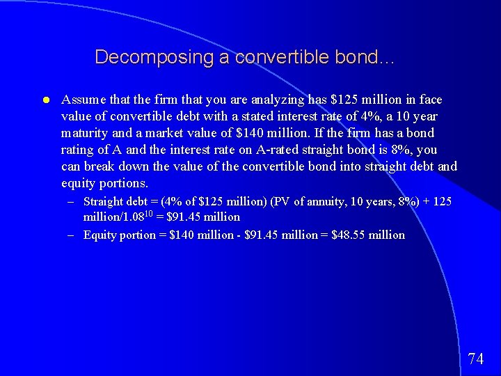
Decomposing a convertible bond… Assume that the firm that you are analyzing has $125 million in face value of convertible debt with a stated interest rate of 4%, a 10 year maturity and a market value of $140 million. If the firm has a bond rating of A and the interest rate on A-rated straight bond is 8%, you can break down the value of the convertible bond into straight debt and equity portions. – Straight debt = (4% of $125 million) (PV of annuity, 10 years, 8%) + 125 million/1. 0810 = $91. 45 million – Equity portion = $140 million - $91. 45 million = $48. 55 million 74

Recapping the Cost of Capital 75

II. Estimating Cash Flows DCF Valuation 76

Steps in Cash Flow Estimation Estimate the current earnings of the firm – If looking at cash flows to equity, look at earnings after interest expenses i. e. net income – If looking at cash flows to the firm, look at operating earnings after taxes Consider how much the firm invested to create future growth – If the investment is not expensed, it will be categorized as capital expenditures. To the extent that depreciation provides a cash flow, it will cover some of these expenditures. – Increasing working capital needs are also investments for future growth If looking at cash flows to equity, consider the cash flows from net debt issues (debt issued - debt repaid) 77

Measuring Cash Flows 78

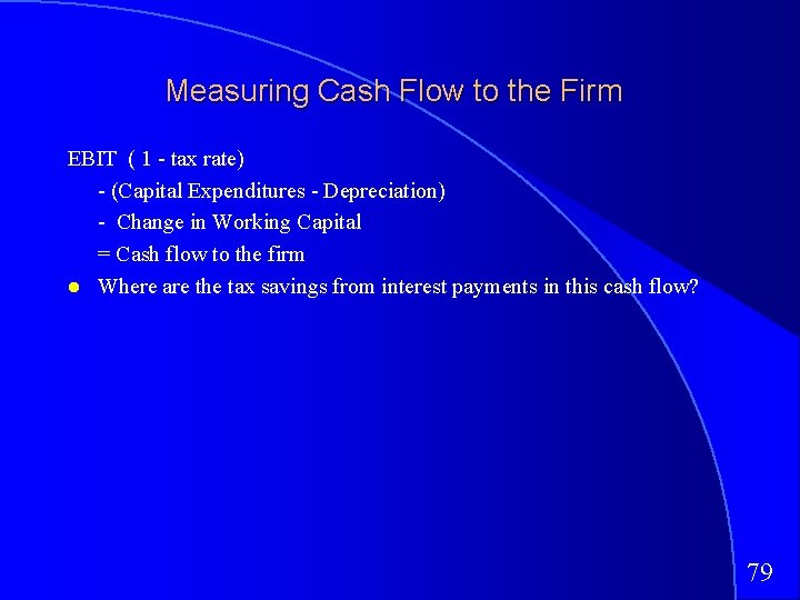
Measuring Cash Flow to the Firm EBIT ( 1 - tax rate) - (Capital Expenditures - Depreciation) - Change in Working Capital = Cash flow to the firm Where are the tax savings from interest payments in this cash flow? 79

From Reported to Actual Earnings 80

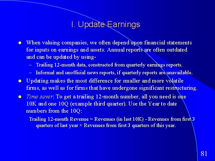
I. Update Earnings When valuing companies, we often depend upon financial statements for inputs on earnings and assets. Annual reports are often outdated and can be updated by using– Trailing 12 -month data, constructed from quarterly earnings reports. – Informal and unofficial news reports, if quarterly reports are unavailable. Updating makes the most difference for smaller and more volatile firms, as well as for firms that have undergone significant restructuring. Time saver: To get a trailing 12 -month number, all you need is one 10 K and one 10 Q (example third quarter). Use the Year to date numbers from the 10 Q: Trailing 12 -month Revenue = Revenues (in last 10 K) - Revenues from first 3 quarters of last year + Revenues from first 3 quarters of this year. 81

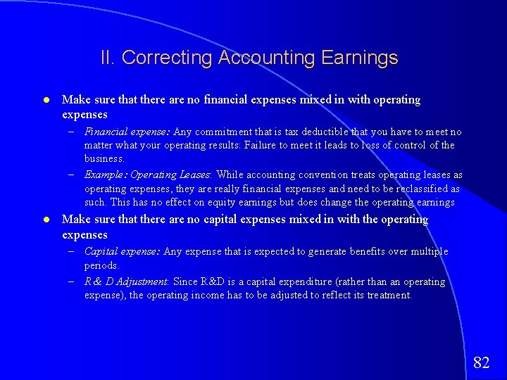
II. Correcting Accounting Earnings Make sure that there are no financial expenses mixed in with operating expenses – Financial expense: Any commitment that is tax deductible that you have to meet no matter what your operating results: Failure to meet it leads to loss of control of the business. – Example: Operating Leases: While accounting convention treats operating leases as operating expenses, they are really financial expenses and need to be reclassified as such. This has no effect on equity earnings but does change the operating earnings Make sure that there are no capital expenses mixed in with the operating expenses – Capital expense: Any expense that is expected to generate benefits over multiple periods. – R & D Adjustment: Since R&D is a capital expenditure (rather than an operating expense), the operating income has to be adjusted to reflect its treatment. 82

The Magnitude of Operating Leases 83

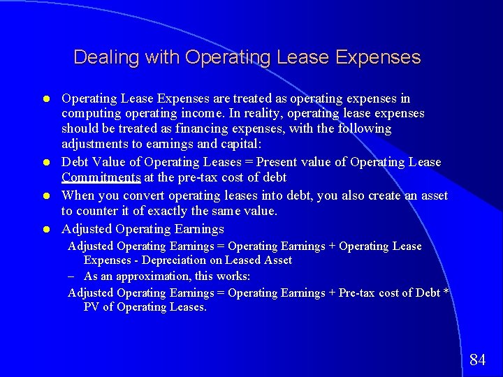
Dealing with Operating Lease Expenses are treated as operating expenses in computing operating income. In reality, operating lease expenses should be treated as financing expenses, with the following adjustments to earnings and capital: Debt Value of Operating Leases = Present value of Operating Lease Commitments at the pre-tax cost of debt When you convert operating leases into debt, you also create an asset to counter it of exactly the same value. Adjusted Operating Earnings = Operating Earnings + Operating Lease Expenses - Depreciation on Leased Asset – As an approximation, this works: Adjusted Operating Earnings = Operating Earnings + Pre-tax cost of Debt * PV of Operating Leases. 84

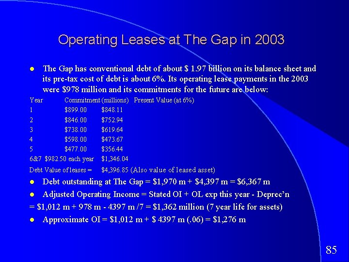
Operating Leases at The Gap in 2003 The Gap has conventional debt of about $ 1. 97 billion on its balance sheet and its pre-tax cost of debt is about 6%. Its operating lease payments in the 2003 were $978 million and its commitments for the future are below: Year Commitment (millions) Present Value (at 6%) 1 $899. 00 $848. 11 2 $846. 00 $752. 94 3 $738. 00 $619. 64 4 $598. 00 $473. 67 5 $477. 00 $356. 44 6&7 $982. 50 each year $1, 346. 04 Debt Value of leases = $4, 396. 85 (Also value of leased asset) Debt outstanding at The Gap = $1, 970 m + $4, 397 m = $6, 367 m Adjusted Operating Income = Stated OI + OL exp this year - Deprec’n = $1, 012 m + 978 m - 4397 m /7 = $1, 362 million (7 year life for assets) Approximate OI = $1, 012 m + $ 4397 m (. 06) = $1, 276 m 85

The Collateral Effects of Treating Operating Leases as Debt 86

The Magnitude of R&D Expenses 87

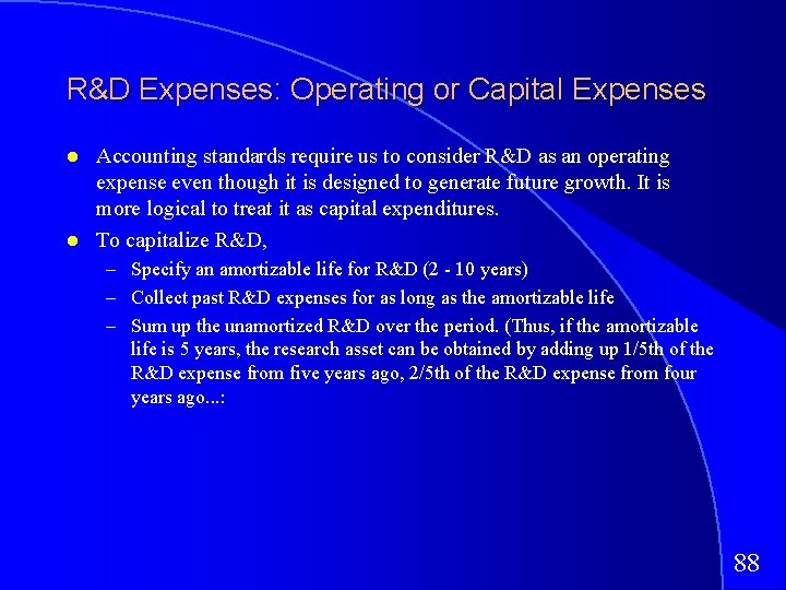
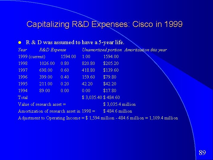
R&D Expenses: Operating or Capital Expenses Accounting standards require us to consider R&D as an operating expense even though it is designed to generate future growth. It is more logical to treat it as capital expenditures. To capitalize R&D, – Specify an amortizable life for R&D (2 - 10 years) – Collect past R&D expenses for as long as the amortizable life – Sum up the unamortized R&D over the period. (Thus, if the amortizable life is 5 years, the research asset can be obtained by adding up 1/5 th of the R&D expense from five years ago, 2/5 th of the R&D expense from four years ago. . . : 88

Capitalizing R&D Expenses: Cisco in 1999 R & D was assumed to have a 5 -year life. Year R&D Expense Unamortized portion Amortization this year 1999 (current) 1594. 00 1998 1026. 00 0. 80 820. 80 $205. 20 1997 698. 00 0. 60 418. 80 $139. 60 1996 399. 00 0. 40 159. 60 $79. 80 1995 211. 00 0. 20 42. 20 $42. 20 1994 89. 00 0. 00 $17. 80 Total $ 3, 035. 40 $ 484. 60 Value of research asset = $ 3, 035. 4 million Amortization of research asset in 1998 = $ 484. 6 million Adjustment to Operating Income = $ 1, 594 million - 484. 6 million = 1, 109. 4 million 89

The Effect of Capitalizing R&D 90

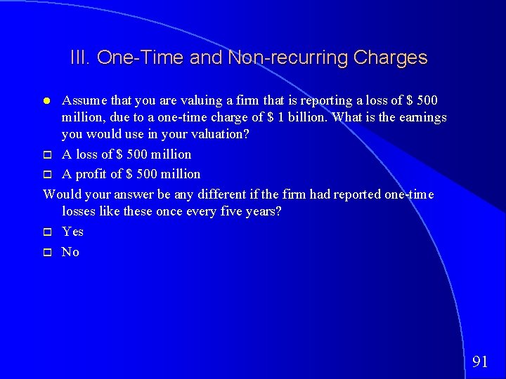
III. One-Time and Non-recurring Charges Assume that you are valuing a firm that is reporting a loss of $ 500 million, due to a one-time charge of $ 1 billion. What is the earnings you would use in your valuation? A loss of $ 500 million A profit of $ 500 million Would your answer be any different if the firm had reported one-time losses like these once every five years? Yes No 91

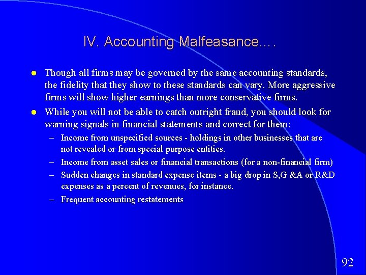
IV. Accounting Malfeasance…. Though all firms may be governed by the same accounting standards, the fidelity that they show to these standards can vary. More aggressive firms will show higher earnings than more conservative firms. While you will not be able to catch outright fraud, you should look for warning signals in financial statements and correct for them: – Income from unspecified sources - holdings in other businesses that are not revealed or from special purpose entities. – Income from asset sales or financial transactions (for a non-financial firm) – Sudden changes in standard expense items - a big drop in S, G &A or R&D expenses as a percent of revenues, for instance. – Frequent accounting restatements 92

V. Dealing with Negative or Abnormally Low Earnings 93

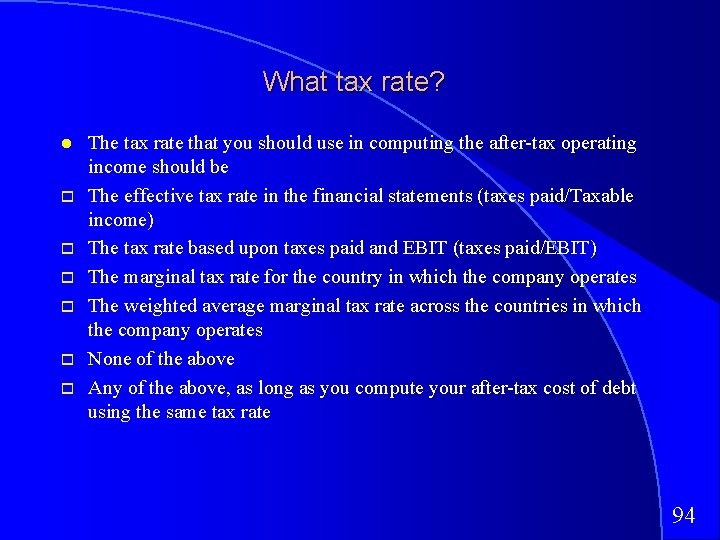
What tax rate? The tax rate that you should use in computing the after-tax operating income should be The effective tax rate in the financial statements (taxes paid/Taxable income) The tax rate based upon taxes paid and EBIT (taxes paid/EBIT) The marginal tax rate for the country in which the company operates The weighted average marginal tax rate across the countries in which the company operates None of the above Any of the above, as long as you compute your after-tax cost of debt using the same tax rate 94

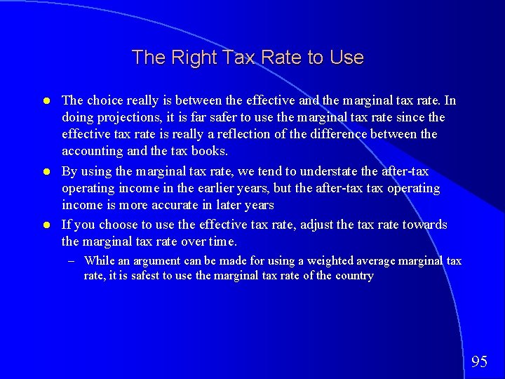
The Right Tax Rate to Use The choice really is between the effective and the marginal tax rate. In doing projections, it is far safer to use the marginal tax rate since the effective tax rate is really a reflection of the difference between the accounting and the tax books. By using the marginal tax rate, we tend to understate the after-tax operating income in the earlier years, but the after-tax operating income is more accurate in later years If you choose to use the effective tax rate, adjust the tax rate towards the marginal tax rate over time. – While an argument can be made for using a weighted average marginal tax rate, it is safest to use the marginal tax rate of the country 95

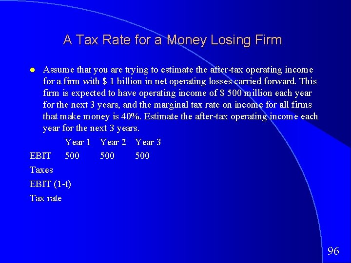
A Tax Rate for a Money Losing Firm Assume that you are trying to estimate the after-tax operating income for a firm with $ 1 billion in net operating losses carried forward. This firm is expected to have operating income of $ 500 million each year for the next 3 years, and the marginal tax rate on income for all firms that make money is 40%. Estimate the after-tax operating income each year for the next 3 years. Year 1 Year 2 Year 3 EBIT 500 500 Taxes EBIT (1 -t) Tax rate 96

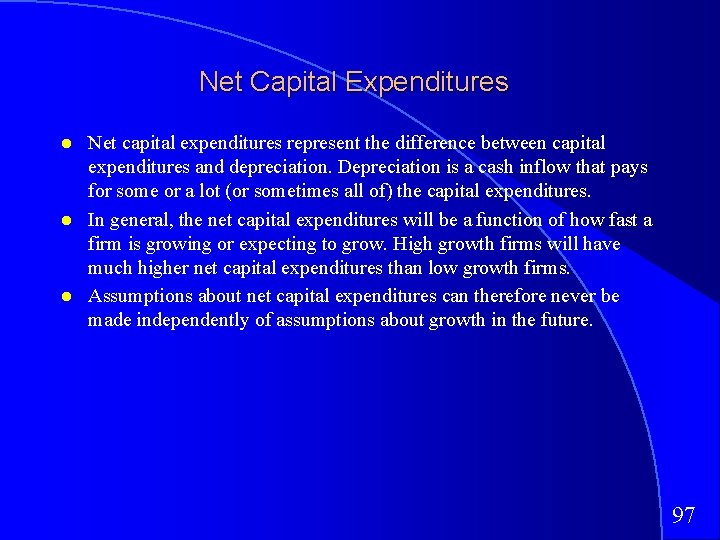
Net Capital Expenditures Net capital expenditures represent the difference between capital expenditures and depreciation. Depreciation is a cash inflow that pays for some or a lot (or sometimes all of) the capital expenditures. In general, the net capital expenditures will be a function of how fast a firm is growing or expecting to grow. High growth firms will have much higher net capital expenditures than low growth firms. Assumptions about net capital expenditures can therefore never be made independently of assumptions about growth in the future. 97

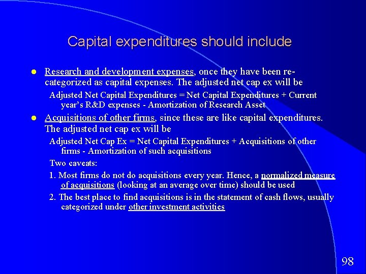
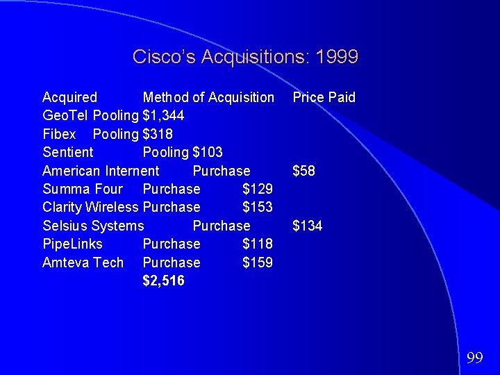
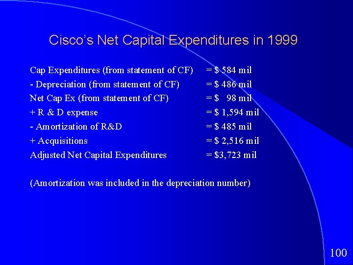
Capital expenditures should include Research and development expenses, once they have been recategorized as capital expenses. The adjusted net cap ex will be Adjusted Net Capital Expenditures = Net Capital Expenditures + Current year’s R&D expenses - Amortization of Research Asset Acquisitions of other firms, since these are like capital expenditures. The adjusted net cap ex will be Adjusted Net Cap Ex = Net Capital Expenditures + Acquisitions of other firms - Amortization of such acquisitions Two caveats: 1. Most firms do not do acquisitions every year. Hence, a normalized measure of acquisitions (looking at an average over time) should be used 2. The best place to find acquisitions is in the statement of cash flows, usually categorized under other investment activities 98

Cisco’s Acquisitions: 1999 Acquired Method of Acquisition Geo. Tel Pooling $1, 344 Fibex Pooling $318 Sentient Pooling $103 American Internent Purchase Summa Four Purchase $129 Clarity Wireless Purchase $153 Selsius Systems Purchase Pipe. Links Purchase $118 Amteva Tech Purchase $159 $2, 516 Price Paid $58 $134 99

Cisco’s Net Capital Expenditures in 1999 Cap Expenditures (from statement of CF) - Depreciation (from statement of CF) Net Cap Ex (from statement of CF) + R & D expense - Amortization of R&D + Acquisitions Adjusted Net Capital Expenditures = $ 584 mil = $ 486 mil = $ 98 mil = $ 1, 594 mil = $ 485 mil = $ 2, 516 mil = $3, 723 mil (Amortization was included in the depreciation number) 100

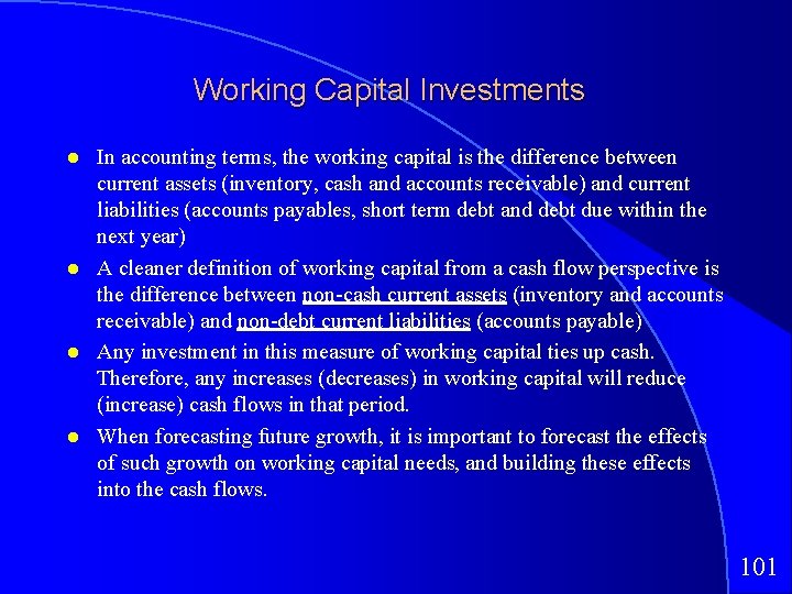
Working Capital Investments In accounting terms, the working capital is the difference between current assets (inventory, cash and accounts receivable) and current liabilities (accounts payables, short term debt and debt due within the next year) A cleaner definition of working capital from a cash flow perspective is the difference between non-cash current assets (inventory and accounts receivable) and non-debt current liabilities (accounts payable) Any investment in this measure of working capital ties up cash. Therefore, any increases (decreases) in working capital will reduce (increase) cash flows in that period. When forecasting future growth, it is important to forecast the effects of such growth on working capital needs, and building these effects into the cash flows. 101

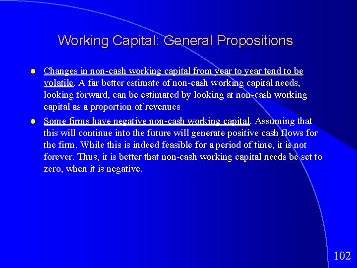
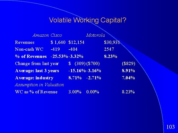
Working Capital: General Propositions Changes in non-cash working capital from year to year tend to be volatile. A far better estimate of non-cash working capital needs, looking forward, can be estimated by looking at non-cash working capital as a proportion of revenues Some firms have negative non-cash working capital. Assuming that this will continue into the future will generate positive cash flows for the firm. While this is indeed feasible for a period of time, it is not forever. Thus, it is better that non-cash working capital needs be set to zero, when it is negative. 102

Volatile Working Capital? Amazon Cisco Motorola Revenues $ 1, 640 $12, 154 $30, 931 Non-cash WC -419 -404 2547 % of Revenues -25. 53%-3. 32% 8. 23% Change from last year $ (309) ($700) Average: last 3 years -15. 16%-3. 16% Average: industry 8. 71% -2. 71% Assumption in Valuation WC as % of Revenue 3. 00% 0. 00% ($829) 8. 91% 7. 04% 8. 23% 103

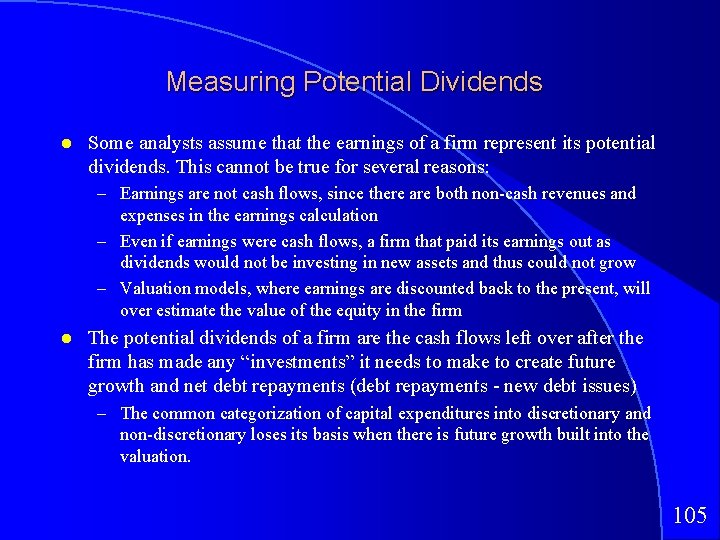
Dividends and Cash Flows to Equity In the strictest sense, the only cash flow that an investor will receive from an equity investment in a publicly traded firm is the dividend that will be paid on the stock. Actual dividends, however, are set by the managers of the firm and may be much lower than the potential dividends (that could have been paid out) – managers are conservative and try to smooth out dividends – managers like to hold on to cash to meet unforeseen future contingencies and investment opportunities When actual dividends are less than potential dividends, using a model that focuses only on dividends will under state the true value of the equity in a firm. 104

Measuring Potential Dividends Some analysts assume that the earnings of a firm represent its potential dividends. This cannot be true for several reasons: – Earnings are not cash flows, since there are both non-cash revenues and expenses in the earnings calculation – Even if earnings were cash flows, a firm that paid its earnings out as dividends would not be investing in new assets and thus could not grow – Valuation models, where earnings are discounted back to the present, will over estimate the value of the equity in the firm The potential dividends of a firm are the cash flows left over after the firm has made any “investments” it needs to make to create future growth and net debt repayments (debt repayments - new debt issues) – The common categorization of capital expenditures into discretionary and non-discretionary loses its basis when there is future growth built into the valuation. 105

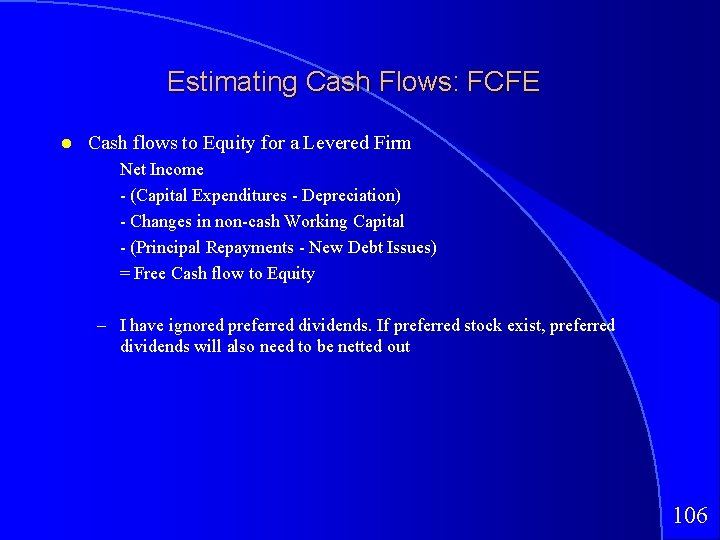
Estimating Cash Flows: FCFE Cash flows to Equity for a Levered Firm Net Income - (Capital Expenditures - Depreciation) - Changes in non-cash Working Capital - (Principal Repayments - New Debt Issues) = Free Cash flow to Equity – I have ignored preferred dividends. If preferred stock exist, preferred dividends will also need to be netted out 106

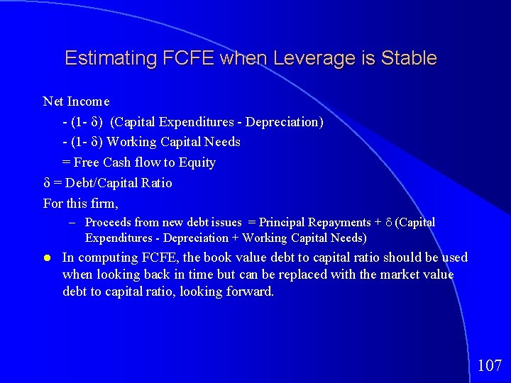
Estimating FCFE when Leverage is Stable Net Income - (1 - ) (Capital Expenditures - Depreciation) - (1 - ) Working Capital Needs = Free Cash flow to Equity = Debt/Capital Ratio For this firm, – Proceeds from new debt issues = Principal Repayments + (Capital Expenditures - Depreciation + Working Capital Needs) In computing FCFE, the book value debt to capital ratio should be used when looking back in time but can be replaced with the market value debt to capital ratio, looking forward. 107

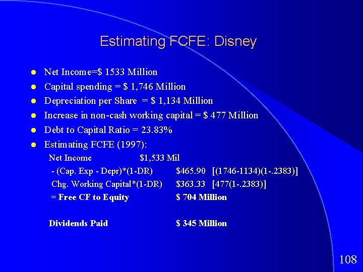
Estimating FCFE: Disney Net Income=$ 1533 Million Capital spending = $ 1, 746 Million Depreciation per Share = $ 1, 134 Million Increase in non-cash working capital = $ 477 Million Debt to Capital Ratio = 23. 83% Estimating FCFE (1997): Net Income $1, 533 Mil - (Cap. Exp - Depr)*(1 -DR) $465. 90 [(1746 -1134)(1 -. 2383)] Chg. Working Capital*(1 -DR) $363. 33 [477(1 -. 2383)] = Free CF to Equity $ 704 Million Dividends Paid $ 345 Million 108

FCFE and Leverage: Is this a free lunch? 109

FCFE and Leverage: The Other Shoe Drops 110

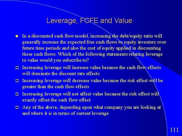
Leverage, FCFE and Value In a discounted cash flow model, increasing the debt/equity ratio will generally increase the expected free cash flows to equity investors over future time periods and also the cost of equity applied in discounting these cash flows. Which of the following statements relating leverage to value would you subscribe to? Increasing leverage will increase value because the cash flow effects will dominate the discount rate effects Increasing leverage will decrease value because the risk effect will be greater than the cash flow effects Increasing leverage will not affect value because the risk effect will exactly offset the cash flow effect Any of the above, depending upon what company you are looking at and where it is in terms of current leverage 111

III. Estimating Growth DCF Valuation 112

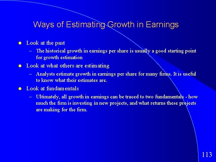
Ways of Estimating Growth in Earnings Look at the past – The historical growth in earnings per share is usually a good starting point for growth estimation Look at what others are estimating – Analysts estimate growth in earnings per share for many firms. It is useful to know what their estimates are. Look at fundamentals – Ultimately, all growth in earnings can be traced to two fundamentals - how much the firm is investing in new projects, and what returns these projects are making for the firm. 113

I. Historical Growth in EPS Historical growth rates can be estimated in a number of different ways – Arithmetic versus Geometric Averages – Simple versus Regression Models Historical growth rates can be sensitive to – the period used in the estimation In using historical growth rates, the following factors have to be considered – how to deal with negative earnings – the effect of changing size 114

Motorola: Arithmetic versus Geometric Growth Rates 115

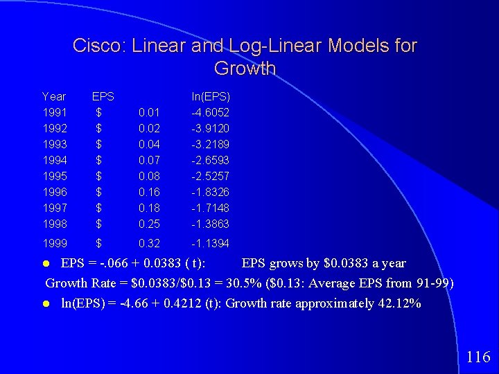
Cisco: Linear and Log-Linear Models for Growth Year 1991 1992 1993 1994 1995 1996 1997 1998 EPS $ $ $ $ 0. 01 0. 02 0. 04 0. 07 0. 08 0. 16 0. 18 0. 25 ln(EPS) -4. 6052 -3. 9120 -3. 2189 -2. 6593 -2. 5257 -1. 8326 -1. 7148 -1. 3863 1999 $ 0. 32 -1. 1394 EPS = -. 066 + 0. 0383 ( t): EPS grows by $0. 0383 a year Growth Rate = $0. 0383/$0. 13 = 30. 5% ($0. 13: Average EPS from 91 -99) ln(EPS) = -4. 66 + 0. 4212 (t): Growth rate approximately 42. 12% 116

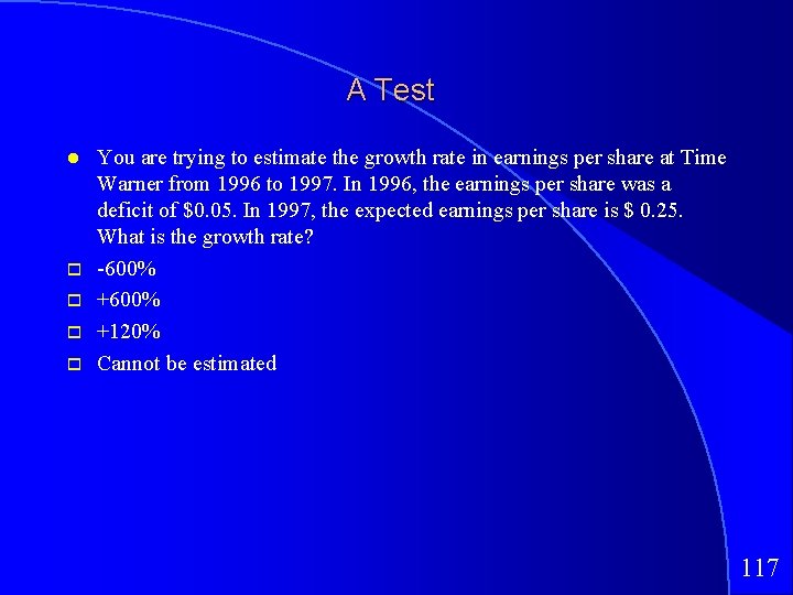
A Test You are trying to estimate the growth rate in earnings per share at Time Warner from 1996 to 1997. In 1996, the earnings per share was a deficit of $0. 05. In 1997, the expected earnings per share is $ 0. 25. What is the growth rate? -600% +120% Cannot be estimated 117

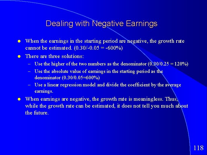
Dealing with Negative Earnings When the earnings in the starting period are negative, the growth rate cannot be estimated. (0. 30/-0. 05 = -600%) There are three solutions: – Use the higher of the two numbers as the denominator (0. 30/0. 25 = 120%) – Use the absolute value of earnings in the starting period as the denominator (0. 30/0. 05=600%) – Use a linear regression model and divide the coefficient by the average earnings. When earnings are negative, the growth rate is meaningless. Thus, while the growth rate can be estimated, it does not tell you much about the future. 118

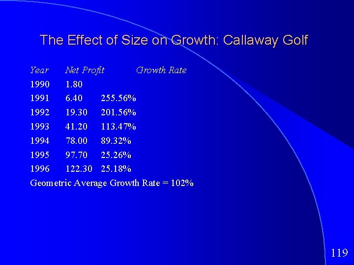
The Effect of Size on Growth: Callaway Golf Year Net Profit Growth Rate 1990 1. 80 1991 6. 40 255. 56% 1992 19. 30 201. 56% 1993 41. 20 113. 47% 1994 78. 00 89. 32% 1995 97. 70 25. 26% 1996 122. 30 25. 18% Geometric Average Growth Rate = 102% 119

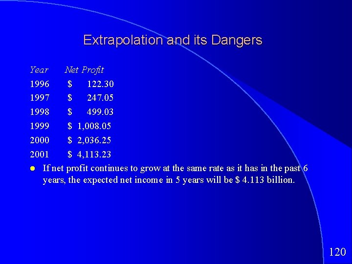
Extrapolation and its Dangers Year Net Profit 1996 $ 122. 30 1997 $ 247. 05 1998 $ 499. 03 1999 $ 1, 008. 05 2000 $ 2, 036. 25 2001 $ 4, 113. 23 If net profit continues to grow at the same rate as it has in the past 6 years, the expected net income in 5 years will be $ 4. 113 billion. 120

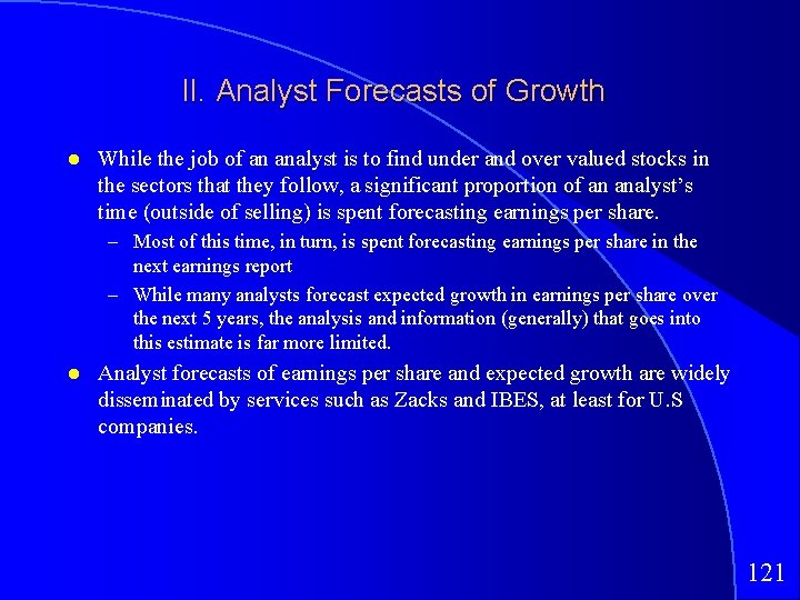
II. Analyst Forecasts of Growth While the job of an analyst is to find under and over valued stocks in the sectors that they follow, a significant proportion of an analyst’s time (outside of selling) is spent forecasting earnings per share. – Most of this time, in turn, is spent forecasting earnings per share in the next earnings report – While many analysts forecast expected growth in earnings per share over the next 5 years, the analysis and information (generally) that goes into this estimate is far more limited. Analyst forecasts of earnings per share and expected growth are widely disseminated by services such as Zacks and IBES, at least for U. S companies. 121

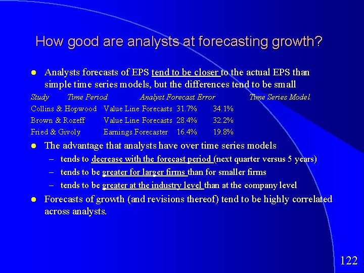
How good are analysts at forecasting growth? Analysts forecasts of EPS tend to be closer to the actual EPS than simple time series models, but the differences tend to be small Study Time Period Analyst Forecast Error Collins & Hopwood Value Line Forecasts 31. 7% 34. 1% Brown & Rozeff Value Line Forecasts 28. 4% 32. 2% Fried & Givoly Earnings Forecaster 16. 4% 19. 8% Time Series Model The advantage that analysts have over time series models – tends to decrease with the forecast period (next quarter versus 5 years) – tends to be greater for larger firms than for smaller firms – tends to be greater at the industry level than at the company level Forecasts of growth (and revisions thereof) tend to be highly correlated across analysts. 122

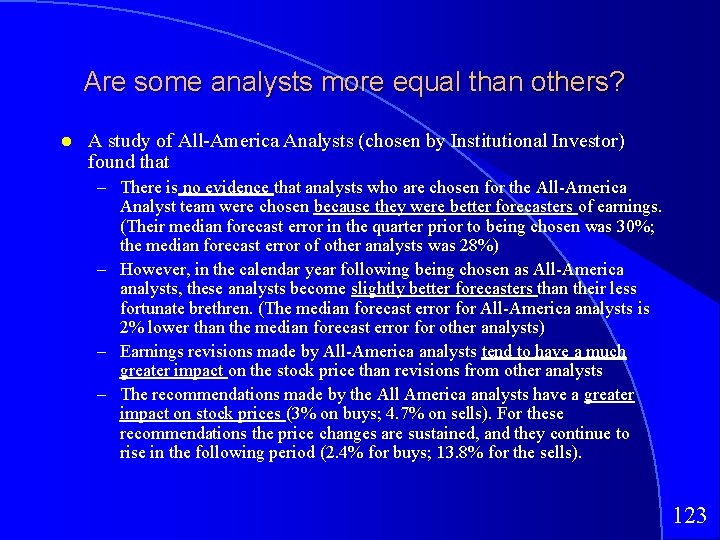
Are some analysts more equal than others? A study of All-America Analysts (chosen by Institutional Investor) found that – There is no evidence that analysts who are chosen for the All-America Analyst team were chosen because they were better forecasters of earnings. (Their median forecast error in the quarter prior to being chosen was 30%; the median forecast error of other analysts was 28%) – However, in the calendar year following being chosen as All-America analysts, these analysts become slightly better forecasters than their less fortunate brethren. (The median forecast error for All-America analysts is 2% lower than the median forecast error for other analysts) – Earnings revisions made by All-America analysts tend to have a much greater impact on the stock price than revisions from other analysts – The recommendations made by the All America analysts have a greater impact on stock prices (3% on buys; 4. 7% on sells). For these recommendations the price changes are sustained, and they continue to rise in the following period (2. 4% for buys; 13. 8% for the sells). 123

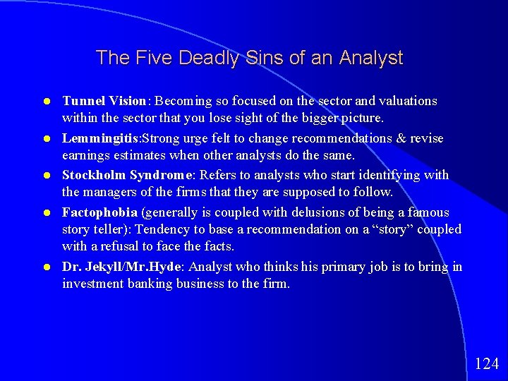
The Five Deadly Sins of an Analyst Tunnel Vision: Becoming so focused on the sector and valuations within the sector that you lose sight of the bigger picture. Lemmingitis: Strong urge felt to change recommendations & revise earnings estimates when other analysts do the same. Stockholm Syndrome: Refers to analysts who start identifying with the managers of the firms that they are supposed to follow. Factophobia (generally is coupled with delusions of being a famous story teller): Tendency to base a recommendation on a “story” coupled with a refusal to face the facts. Dr. Jekyll/Mr. Hyde: Analyst who thinks his primary job is to bring in investment banking business to the firm. 124

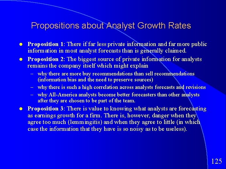
Propositions about Analyst Growth Rates Proposition 1: There if far less private information and far more public information in most analyst forecasts than is generally claimed. Proposition 2: The biggest source of private information for analysts remains the company itself which might explain – why there are more buy recommendations than sell recommendations (information bias and the need to preserve sources) – why there is such a high correlation across analysts forecasts and revisions – why All-America analysts become better forecasters than other analysts after they are chosen to be part of the team. Proposition 3: There is value to knowing what analysts are forecasting as earnings growth for a firm. There is, however, danger when they agree too much (lemmingitis) and when they agree to little (in which case the information that they have is so noisy as to be useless). 125

III. Fundamental Growth Rates 126

Growth Rate Derivations 127

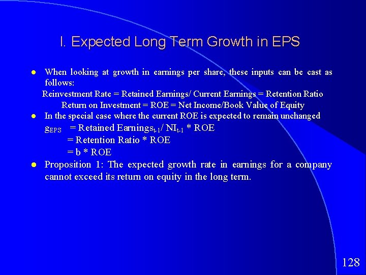
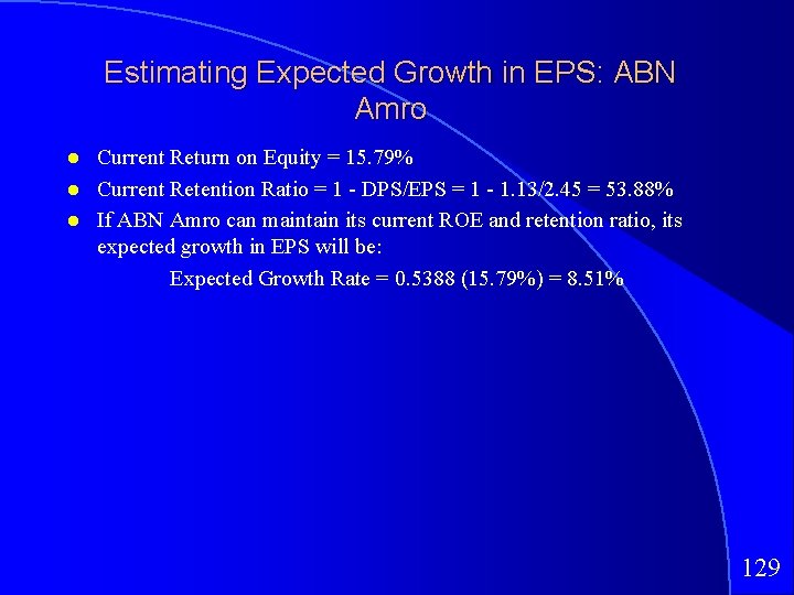
I. Expected Long Term Growth in EPS When looking at growth in earnings per share, these inputs can be cast as follows: Reinvestment Rate = Retained Earnings/ Current Earnings = Retention Ratio Return on Investment = ROE = Net Income/Book Value of Equity In the special case where the current ROE is expected to remain unchanged g. EPS = Retained Earningst-1/ NIt-1 * ROE = Retention Ratio * ROE = b * ROE Proposition 1: The expected growth rate in earnings for a company cannot exceed its return on equity in the long term. 128

Estimating Expected Growth in EPS: ABN Amro Current Return on Equity = 15. 79% Current Retention Ratio = 1 - DPS/EPS = 1 - 1. 13/2. 45 = 53. 88% If ABN Amro can maintain its current ROE and retention ratio, its expected growth in EPS will be: Expected Growth Rate = 0. 5388 (15. 79%) = 8. 51% 129

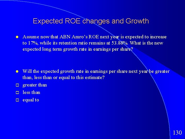
Expected ROE changes and Growth Assume now that ABN Amro’s ROE next year is expected to increase to 17%, while its retention ratio remains at 53. 88%. What is the new expected long term growth rate in earnings per share? Will the expected growth rate in earnings per share next year be greater than, less than or equal to this estimate? greater than less than equal to 130

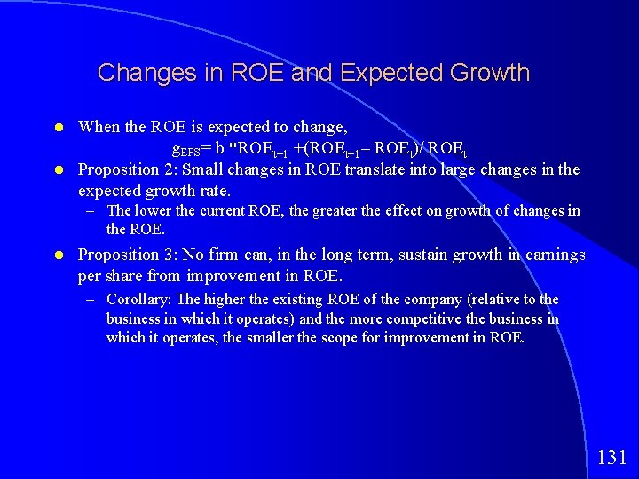
Changes in ROE and Expected Growth When the ROE is expected to change, g. EPS= b *ROEt+1 +(ROEt+1– ROEt)/ ROEt Proposition 2: Small changes in ROE translate into large changes in the expected growth rate. – The lower the current ROE, the greater the effect on growth of changes in the ROE. Proposition 3: No firm can, in the long term, sustain growth in earnings per share from improvement in ROE. – Corollary: The higher the existing ROE of the company (relative to the business in which it operates) and the more competitive the business in which it operates, the smaller the scope for improvement in ROE. 131

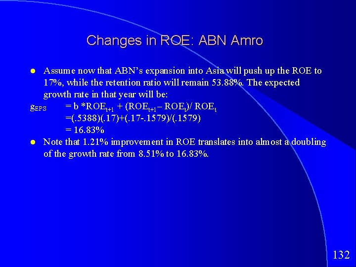
Changes in ROE: ABN Amro Assume now that ABN’s expansion into Asia will push up the ROE to 17%, while the retention ratio will remain 53. 88%. The expected growth rate in that year will be: g. EPS = b *ROEt+1 + (ROEt+1– ROEt)/ ROEt =(. 5388)(. 17)+(. 17 -. 1579)/(. 1579) = 16. 83% Note that 1. 21% improvement in ROE translates into almost a doubling of the growth rate from 8. 51% to 16. 83%. 132

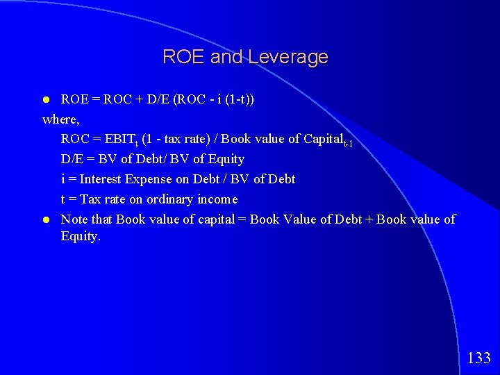
ROE and Leverage ROE = ROC + D/E (ROC - i (1 -t)) where, ROC = EBITt (1 - tax rate) / Book value of Capitalt-1 D/E = BV of Debt/ BV of Equity i = Interest Expense on Debt / BV of Debt t = Tax rate on ordinary income Note that Book value of capital = Book Value of Debt + Book value of Equity. 133

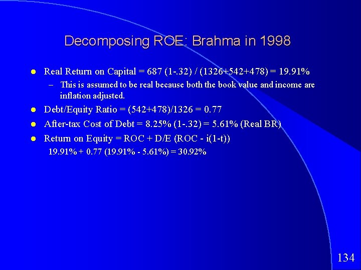
Decomposing ROE: Brahma in 1998 Real Return on Capital = 687 (1 -. 32) / (1326+542+478) = 19. 91% – This is assumed to be real because both the book value and income are inflation adjusted. Debt/Equity Ratio = (542+478)/1326 = 0. 77 After-tax Cost of Debt = 8. 25% (1 -. 32) = 5. 61% (Real BR) Return on Equity = ROC + D/E (ROC - i(1 -t)) 19. 91% + 0. 77 (19. 91% - 5. 61%) = 30. 92% 134

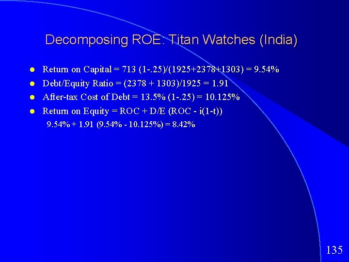
Decomposing ROE: Titan Watches (India) Return on Capital = 713 (1 -. 25)/(1925+2378+1303) = 9. 54% Debt/Equity Ratio = (2378 + 1303)/1925 = 1. 91 After-tax Cost of Debt = 13. 5% (1 -. 25) = 10. 125% Return on Equity = ROC + D/E (ROC - i(1 -t)) 9. 54% + 1. 91 (9. 54% - 10. 125%) = 8. 42% 135

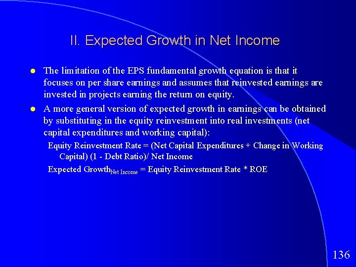
II. Expected Growth in Net Income The limitation of the EPS fundamental growth equation is that it focuses on per share earnings and assumes that reinvested earnings are invested in projects earning the return on equity. A more general version of expected growth in earnings can be obtained by substituting in the equity reinvestment into real investments (net capital expenditures and working capital): Equity Reinvestment Rate = (Net Capital Expenditures + Change in Working Capital) (1 - Debt Ratio)/ Net Income Expected Growth. Net Income = Equity Reinvestment Rate * ROE 136

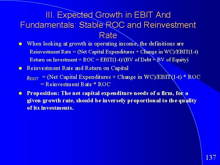
III. Expected Growth in EBIT And Fundamentals: Stable ROC and Reinvestment Rate When looking at growth in operating income, the definitions are Reinvestment Rate = (Net Capital Expenditures + Change in WC)/EBIT(1 -t) Return on Investment = ROC = EBIT(1 -t)/(BV of Debt + BV of Equity) Reinvestment Rate and Return on Capital g. EBIT = (Net Capital Expenditures + Change in WC)/EBIT(1 -t) * ROC = Reinvestment Rate * ROC Proposition: The net capital expenditure needs of a firm, for a given growth rate, should be inversely proportional to the quality of its investments. 137

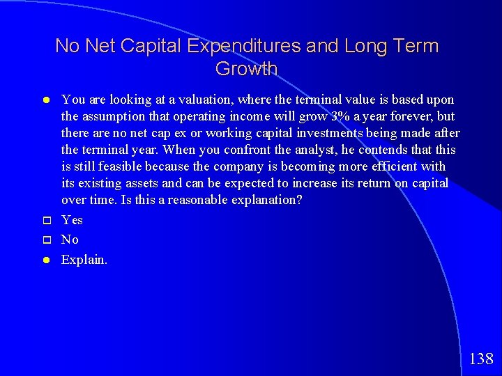
No Net Capital Expenditures and Long Term Growth You are looking at a valuation, where the terminal value is based upon the assumption that operating income will grow 3% a year forever, but there are no net cap ex or working capital investments being made after the terminal year. When you confront the analyst, he contends that this is still feasible because the company is becoming more efficient with its existing assets and can be expected to increase its return on capital over time. Is this a reasonable explanation? Yes No Explain. 138

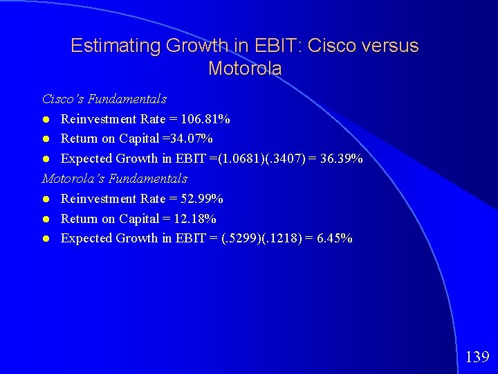
Estimating Growth in EBIT: Cisco versus Motorola Cisco’s Fundamentals Reinvestment Rate = 106. 81% Return on Capital =34. 07% Expected Growth in EBIT =(1. 0681)(. 3407) = 36. 39% Motorola’s Fundamentals Reinvestment Rate = 52. 99% Return on Capital = 12. 18% Expected Growth in EBIT = (. 5299)(. 1218) = 6. 45% 139

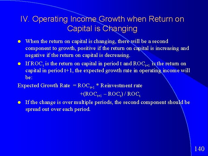
IV. Operating Income Growth when Return on Capital is Changing When the return on capital is changing, there will be a second component to growth, positive if the return on capital is increasing and negative if the return on capital is decreasing. If ROCt is the return on capital in period t and ROCt+1 is the return on capital in period t+1, the expected growth rate in operating income will be: Expected Growth Rate = ROCt+1 * Reinvestment rate +(ROCt+1 – ROCt) / ROCt If the change is over multiple periods, the second component should be spread out over each period. 140

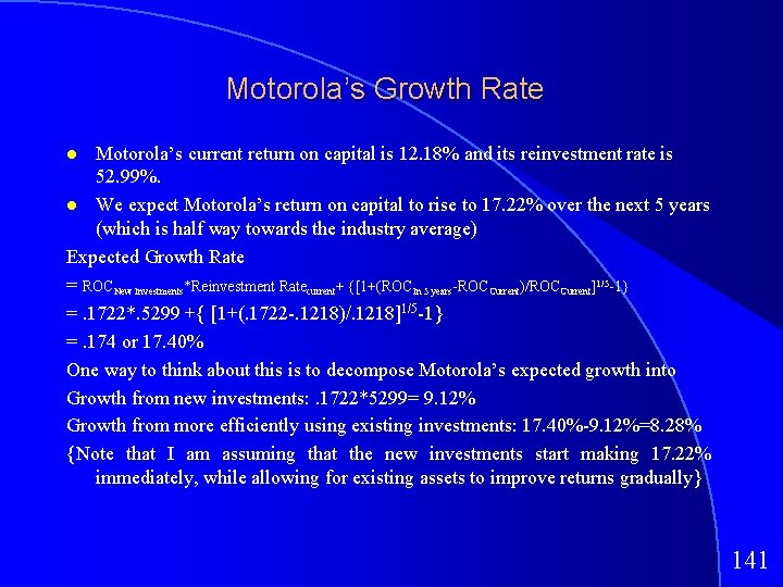
Motorola’s Growth Rate Motorola’s current return on capital is 12. 18% and its reinvestment rate is 52. 99%. We expect Motorola’s return on capital to rise to 17. 22% over the next 5 years (which is half way towards the industry average) Expected Growth Rate = ROCNew Investments*Reinvestment Ratecurrent+ {[1+(ROCIn 5 years-ROCCurrent)/ROCCurrent]1/5 -1} =. 1722*. 5299 +{ [1+(. 1722 -. 1218)/. 1218]1/5 -1} =. 174 or 17. 40% One way to think about this is to decompose Motorola’s expected growth into Growth from new investments: . 1722*5299= 9. 12% Growth from more efficiently using existing investments: 17. 40%-9. 12%=8. 28% {Note that I am assuming that the new investments start making 17. 22% immediately, while allowing for existing assets to improve returns gradually} 141

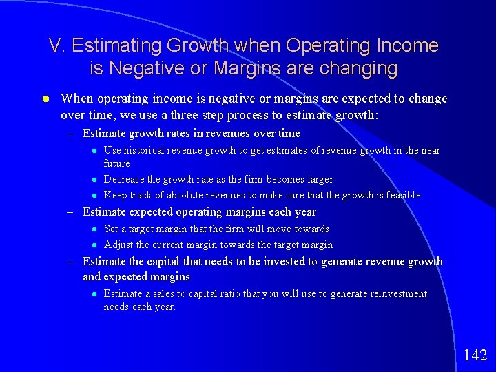
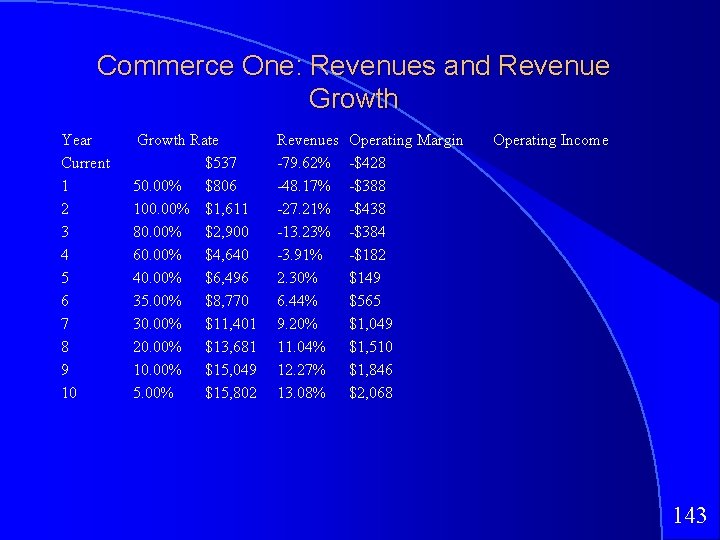
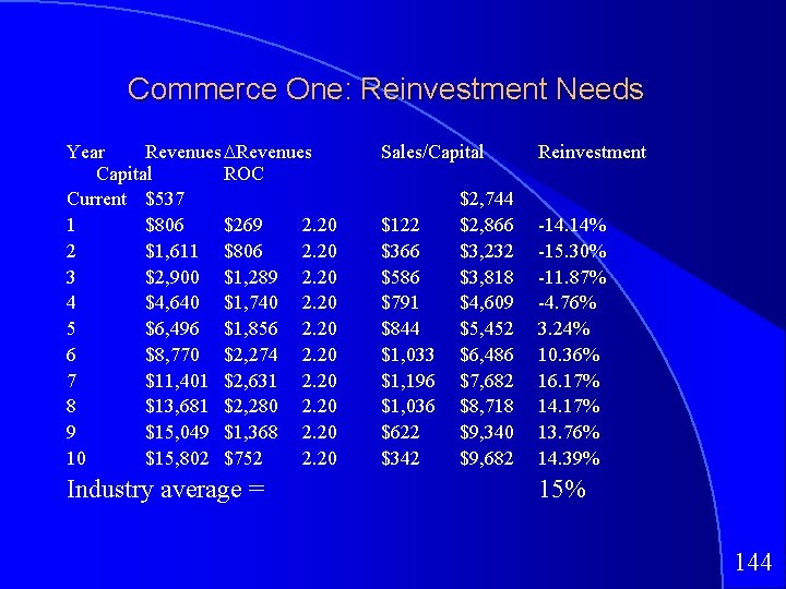
V. Estimating Growth when Operating Income is Negative or Margins are changing When operating income is negative or margins are expected to change over time, we use a three step process to estimate growth: – Estimate growth rates in revenues over time Use historical revenue growth to get estimates of revenue growth in the near future Decrease the growth rate as the firm becomes larger Keep track of absolute revenues to make sure that the growth is feasible – Estimate expected operating margins each year Set a target margin that the firm will move towards Adjust the current margin towards the target margin – Estimate the capital that needs to be invested to generate revenue growth and expected margins Estimate a sales to capital ratio that you will use to generate reinvestment needs each year. 142

Commerce One: Revenues and Revenue Growth Year Current 1 2 3 4 5 6 7 8 9 10 Growth Rate $537 50. 00% $806 100. 00% $1, 611 80. 00% $2, 900 60. 00% $4, 640 40. 00% $6, 496 35. 00% $8, 770 30. 00% $11, 401 20. 00% $13, 681 10. 00% $15, 049 5. 00% $15, 802 Revenues -79. 62% -48. 17% -27. 21% -13. 23% -3. 91% 2. 30% 6. 44% 9. 20% 11. 04% 12. 27% 13. 08% Operating Margin -$428 -$388 -$438 -$384 -$182 $149 $565 $1, 049 $1, 510 $1, 846 $2, 068 Operating Income 143

Commerce One: Reinvestment Needs Year Revenues Capital ROC Current $537 1 $806 $269 2. 20 2 $1, 611 $806 2. 20 3 $2, 900 $1, 289 2. 20 4 $4, 640 $1, 740 2. 20 5 $6, 496 $1, 856 2. 20 6 $8, 770 $2, 274 2. 20 7 $11, 401 $2, 631 2. 20 8 $13, 681 $2, 280 2. 20 9 $15, 049 $1, 368 2. 20 10 $15, 802 $752 2. 20 Industry average = Sales/Capital $122 $366 $586 $791 $844 $1, 033 $1, 196 $1, 036 $622 $342 $2, 744 $2, 866 $3, 232 $3, 818 $4, 609 $5, 452 $6, 486 $7, 682 $8, 718 $9, 340 $9, 682 Reinvestment -14. 14% -15. 30% -11. 87% -4. 76% 3. 24% 10. 36% 16. 17% 14. 17% 13. 76% 14. 39% 15% 144

145

IV. Closure in Valuation Discounted Cashflow Valuation 146

Getting Closure in Valuation A publicly traded firm potentially has an infinite life. The value is therefore the present value of cash flows forever. Since we cannot estimate cash flows forever, we estimate cash flows for a “growth period” and then estimate a terminal value, to capture the value at the end of the period: 147

Ways of Estimating Terminal Value 148

Stable Growth and Terminal Value When a firm’s cash flows grow at a “constant” rate forever, the present value of those cash flows can be written as: Value = Expected Cash Flow Next Period / (r - g) where, r = Discount rate (Cost of Equity or Cost of Capital) g = Expected growth rate This “constant” growth rate is called a stable growth rate and cannot be higher than the growth rate of the economy in which the firm operates. While companies can maintain high growth rates for extended periods, they will approach “stable growth” at some point in time. When they do approach stable growth, the valuation formula above can be used to estimate the “terminal value” of all cash flows beyond. 149

Limits on Stable Growth The stable growth rate cannot exceed the growth rate of the economy but it can be set lower. – If you assume that the economy is composed of high growth and stable growth firms, the growth rate of the latter will probably be lower than the growth rate of the economy. – The stable growth rate can be negative. The terminal value will be lower and you are assuming that your firm will disappear over time. – If you use nominal cashflows and discount rates, the growth rate should be nominal in the currency in which the valuation is denominated. One simple proxy for the nominal growth rate of the economy is the riskfree rate. 150

Growth Patterns A key assumption in all discounted cash flow models is the period of high growth, and the pattern of growth during that period. In general, we can make one of three assumptions: – there is no high growth, in which case the firm is already in stable growth – there will be high growth for a period, at the end of which the growth rate will drop to the stable growth rate (2 -stage) – there will be high growth for a period, at the end of which the growth rate will decline gradually to a stable growth rate(3 -stage) – Each year will have different margins and different growth rates (n stage) 151

Determinants of Growth Patterns Size of the firm – Success usually makes a firm larger. As firms become larger, it becomes much more difficult for them to maintain high growth rates Current growth rate – While past growth is not always a reliable indicator of future growth, there is a correlation between current growth and future growth. Thus, a firm growing at 30% currently probably has higher growth and a longer expected growth period than one growing 10% a year now. Barriers to entry and differential advantages – Ultimately, high growth comes from high project returns, which, in turn, comes from barriers to entry and differential advantages. – The question of how long growth will last and how high it will be can therefore be framed as a question about what the barriers to entry are, how long they will stay up and how strong they will remain. 152

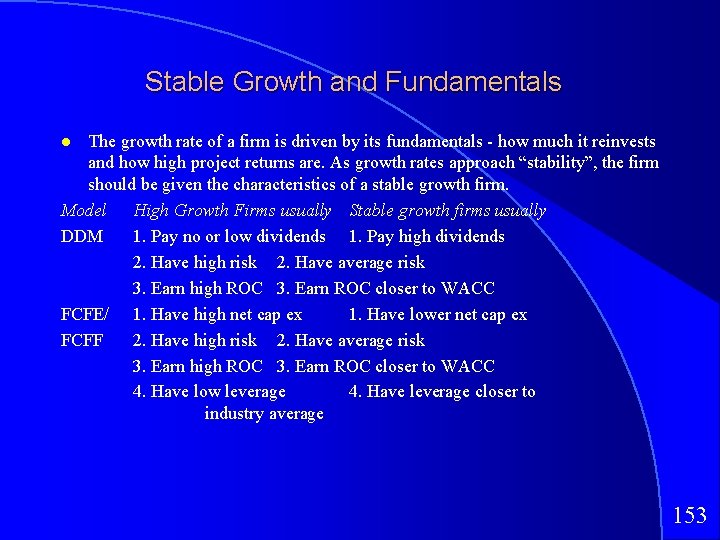
Stable Growth and Fundamentals The growth rate of a firm is driven by its fundamentals - how much it reinvests and how high project returns are. As growth rates approach “stability”, the firm should be given the characteristics of a stable growth firm. Model High Growth Firms usually Stable growth firms usually DDM 1. Pay no or low dividends 1. Pay high dividends 2. Have high risk 2. Have average risk 3. Earn high ROC 3. Earn ROC closer to WACC FCFE/ 1. Have high net cap ex 1. Have lower net cap ex FCFF 2. Have high risk 2. Have average risk 3. Earn high ROC 3. Earn ROC closer to WACC 4. Have low leverage 4. Have leverage closer to industry average 153

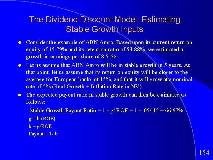
The Dividend Discount Model: Estimating Stable Growth Inputs Consider the example of ABN Amro. Based upon its current return on equity of 15. 79% and its retention ratio of 53. 88%, we estimated a growth in earnings per share of 8. 51%. Let us assume that ABN Amro will be in stable growth in 5 years. At that point, let us assume that its return on equity will be closer to the average for European banks of 15%, and that it will grow at a nominal rate of 5% (Real Growth + Inflation Rate in NV) The expected payout ratio in stable growth can then be estimated as follows: Stable Growth Payout Ratio = 1 - g/ ROE = 1 -. 05/. 15 = 66. 67% g = b (ROE) b = g/ROE Payout = 1 - b 154

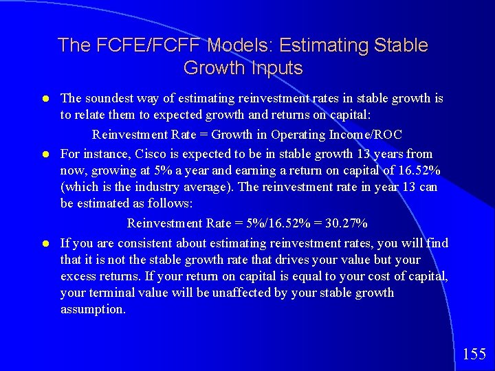
The FCFE/FCFF Models: Estimating Stable Growth Inputs The soundest way of estimating reinvestment rates in stable growth is to relate them to expected growth and returns on capital: Reinvestment Rate = Growth in Operating Income/ROC For instance, Cisco is expected to be in stable growth 13 years from now, growing at 5% a year and earning a return on capital of 16. 52% (which is the industry average). The reinvestment rate in year 13 can be estimated as follows: Reinvestment Rate = 5%/16. 52% = 30. 27% If you are consistent about estimating reinvestment rates, you will find that it is not the stable growth rate that drives your value but your excess returns. If your return on capital is equal to your cost of capital, your terminal value will be unaffected by your stable growth assumption. 155

V. Beyond Inputs: Choosing and Using the Right Model Discounted Cashflow Valuation 156

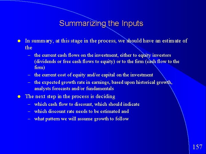
Summarizing the Inputs In summary, at this stage in the process, we should have an estimate of the – the current cash flows on the investment, either to equity investors (dividends or free cash flows to equity) or to the firm (cash flow to the firm) – the current cost of equity and/or capital on the investment – the expected growth rate in earnings, based upon historical growth, analysts forecasts and/or fundamentals The next step in the process is deciding – which cash flow to discount, which should indicate – which discount rate needs to be estimated and – what pattern we will assume growth to follow 157

Which cash flow should I discount? Use Equity Valuation (a) for firms which have stable leverage, whether high or not, and (b) if equity (stock) is being valued Use Firm Valuation (a) for firms which have leverage which is too high or too low, and expect to change the leverage over time, because debt payments and issues do not have to be factored in the cash flows and the discount rate (cost of capital) does not change dramatically over time. (b) for firms for which you have partial information on leverage (eg: interest expenses are missing. . ) (c) in all other cases, where you are more interested in valuing the firm than the equity. (Value Consulting? ) 158

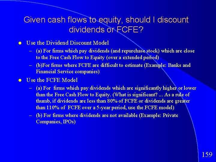
Given cash flows to equity, should I discount dividends or FCFE? Use the Dividend Discount Model – (a) For firms which pay dividends (and repurchase stock) which are close to the Free Cash Flow to Equity (over a extended period) – (b)For firms where FCFE are difficult to estimate (Example: Banks and Financial Service companies) Use the FCFE Model – (a) For firms which pay dividends which are significantly higher or lower than the Free Cash Flow to Equity. (What is significant? . . . As a rule of thumb, if dividends are less than 80% of FCFE or dividends are greater than 110% of FCFE over a 5 -year period, use the FCFE model) – (b) For firms where dividends are not available (Example: Private Companies, IPOs) 159

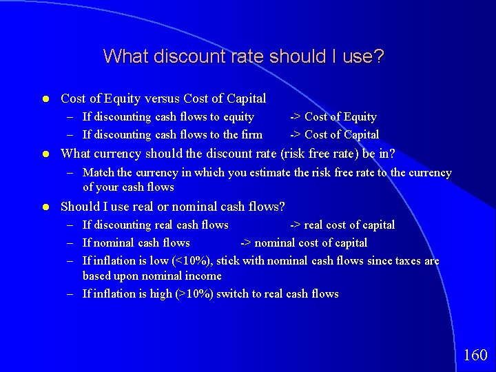
What discount rate should I use? Cost of Equity versus Cost of Capital – If discounting cash flows to equity – If discounting cash flows to the firm -> Cost of Equity -> Cost of Capital What currency should the discount rate (risk free rate) be in? – Match the currency in which you estimate the risk free rate to the currency of your cash flows Should I use real or nominal cash flows? – If discounting real cash flows -> real cost of capital – If nominal cash flows -> nominal cost of capital – If inflation is low (<10%), stick with nominal cash flows since taxes are based upon nominal income – If inflation is high (>10%) switch to real cash flows 160

Which Growth Pattern Should I use? If your firm is – large and growing at a rate close to or less than growth rate of the economy, or – constrained by regulation from growing at rate faster than the economy – has the characteristics of a stable firm (average risk & reinvestment rates) Use a Stable Growth Model If your firm – is large & growing at a moderate (≤ Overall growth rate + 10%) or – has a single product & barriers to entry with a finite life (e. g. patents) Use a 2 -Stage Growth Model If your firm – is small and growing at a very high rate (> Overall growth rate + 10%) or – has significant barriers to entry into the business – has firm characteristics that are very different from the norm Use a 3 -Stage or n-stage Model 161

The Building Blocks of Valuation 162

6. Tying up Loose Ends 163

1. Dealing with Cash and Marketable Securities The simplest and most direct way of dealing with cash and marketable securities is to keep it out of the valuation - the cash flows should be before interest income from cash and securities, and the discount rate should not be contaminated by the inclusion of cash. (Use betas of the operating assets alone to estimate the cost of equity). Once the firm has been valued, add back the value of cash and marketable securities and subtract out gross debt. (This is also equivalent to subtracting out net debt) – If you have a particularly incompetent management, with a history of overpaying on acquisitions, markets may discount the value of this cash. 164

How much cash is too much cash? 165

The Value of Cash Implicitly, we are assuming here that the market will value cash at face value. Assume now that you are buying a firm whose only asset is marketable securities worth $ 100 million. Can you ever consider a scenario where you would not be willing to pay $ 100 million for this firm? Yes No What is or are the scenario(s)? 166

The Case of Closed End Funds Closed end funds are mutual funds, with a fixed number of shares. Unlike regular mutual funds, where the shares have to trade at net asset value (which is the value of the securities in the fund), closed end funds shares can and often do trade at prices which are different from the net asset value. The average closed end fund has always traded at a discount on net asset value (of between 10 and 20%) in the United States. 167

Closed End Funds: Price and NAV 168

A Simple Explanation for the Closed End Discount Assume that you have a closed-end fund that invests in ‘average risk” stocks. Assume also that you expect the market (average risk investments) to make 11. 5% annually over the long term. If the closed end fund underperforms the market by 0. 50%, estimate the discount on the fund. 169

A Premium for Marketable Securities Some closed end funds trade at a premium on net asset value. For instance, the Thai closed end funds were trading at a premium of roughly 40% on net asset value and the Indonesian fund at a premium of 80%+ on NAV on December 31, 1997. Why might an investor be willing to pay a premium over the value of the marketable securities in the fund? 170

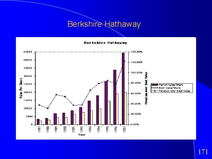
Berkshire Hathaway 171

2. Dealing with Holdings in Other firms Holdings in other firms can be categorized into – Minority passive holdings, in which case only the dividend from the holdings is shown in the balance sheet – Minority active holdings, in which case the share of equity income is shown in the income statements – Majority active holdings, in which case the financial statements are consolidated. 172

An Exercise in Valuing Cross Holdings Assume that you have valued Company A using consolidated financials for $ 1 billion (using FCFF and cost of capital) and that the firm has $ 200 million in debt. How much is the equity in Company A worth? Now assume that you are told that Company A owns 10% of Company B and that the holdings are accounted for as passive holdings. If the market cap of company B is $ 500 million, how much is the equity in Company A worth? Now add on the assumption that Company A owns 60% of Company C and that the holdings are fully consolidated. The minority interest in company C is recorded at $ 40 million in Company A’s balance sheet. How much is the equity in Company A worth? 173

More on Cross Holding Valuation Building on the previous example, assume that – You have valued equity in company B at $ 250 million (which is half the market’s estimate of value currently) – Company A is a steel company and that company C is a chemical company. Furthermore, assume that you have valued the equity in company C at $250 million. Estimate the value of equity in company A. 174

If you really want to value cross holdings right…. Step 1: Value the parent company without any cross holdings. This will require using unconsolidated financial statements rather than consolidated ones. Step 2: Value each of the cross holdings individually. (If you use the market values of the cross holdings, you will build in errors the market makes in valuing them into your valuation. Step 3: The final value of the equity in the parent company with N cross holdings will be: Value of un-consolidated parent company – Debt of un-consolidated parent company + 175

If you have to settle for an approximation, try this… For majority holdings, with full consolidation, convert the minority interest from book value to market value by applying a price to book ratio (based upon the sector average for the subsidiary) to the minority interest. – Estimated market value of minority interest = Minority interest on balance sheet * Price to Book ratio for sector (of subsidiary) – Subtract this from the estimated value of the consolidated firm to get to value of the equity in the parent company. For minority holdings in other companies, convert the book value of these holdings (which are reported on the balance sheet) into market value by multiplying by the price to book ratio of the sector(s). Add this value on to the value of the operating assets to arrive at total firm value. 176

3. Equity Options issued by the firm. . Any options issued by a firm, whether to management or employees or to investors (convertibles and warrants) create claims on the equity of the firm. By creating claims on the equity, they can affect the value of equity per share. Failing to fully take into account this claim on the equity in valuation will result in an overstatement of the value of equity per share. 177

Why do options affect equity value per share? It is true that options can increase the number of shares outstanding but dilution per se is not the problem. Options affect equity value because – Shares are issued at below the prevailing market price. Options get exercised only when they are in the money. – Alternatively, the company can use cashflows that would have been available to equity investors to buy back shares which are then used to meet option exercise. The lower cashflows reduce equity value. 178

A simple example… XYZ company has $ 100 million in free cashflows to the firm, growing 3% a year in perpetuity and a cost of capital of 8%. It has 100 million shares outstanding and $ 1 billion in debt. Its value can be written as follows: Value of firm = 100 / (. 08 -. 03) - Debt = Equity Value per share = 2000 = 1000/100 = $10 179

Now come the options… XYZ decides to give 10 million options at the money (with a strike price of $10) to its CEO. What effect will this have on the value of equity per share? a) None. The options are not in-the-money. b) Decrease by 10%, since the number of shares could increase by 10 million c) Decrease by less than 10%. The options will bring in cash into the firm but they have time value. 180

Dealing with Employee Options: The Bludgeon Approach The simplest way of dealing with options is to try to adjust the denominator for shares that will become outstanding if the options get exercised. In the example cited, this would imply the following: Value of firm = 100 / (. 08 -. 03) - Debt = Equity Number of diluted shares Value per share = 2000 = 1000 = 110 = 1000/110 = $9. 09 181

Problem with the diluted approach The diluted approach fails to consider that exercising options will bring in cash into the firm. Consequently, they will overestimate the impact of options and understate the value of equity per share. The degree to which the approach will understate value will depend upon how high the exercise price is relative to the market price. In cases where the exercise price is a fraction of the prevailing market price, the diluted approach will give you a reasonable estimate of value per share. 182

The Treasury Stock Approach The treasury stock approach adds the proceeds from the exercise of options to the value of the equity before dividing by the diluted number of shares outstanding. In the example cited, this would imply the following: Value of firm = 100 / (. 08 -. 03) - Debt = Equity Number of diluted shares Proceeds from option exercise Value per share = 2000 = 1000 = 110 = 10 * 10 = 100 (Exercise price = 10) = (1000+ 100)/110 = $ 10 183

Problems with the treasury stock approach The treasury stock approach fails to consider the time premium on the options. In the example used, we are assuming that an at the money option is essentially worth nothing. The treasury stock approach also has problems with out-of-the-money options. If considered, they can increase the value of equity per share. If ignored, they are treated as non-existent. 184

Dealing with options the right way… Step 1: Value the firm, using discounted cash flow or other valuation models. Step 2: Subtract out the value of the outstanding debt to arrive at the value of equity. Alternatively, skip step 1 and estimate the of equity directly. Step 3: Subtract out the market value (or estimated market value) of other equity claims: – Value of Warrants = Market Price per Warrant * Number of Warrants : Alternatively estimate the value using option pricing model – Value of Conversion Option = Market Value of Convertible Bonds - Value of Straight Debt Portion of Convertible Bonds – Value of employee Options: Value using the average exercise price and maturity. Step 4: Divide the remaining value of equity by the number of shares outstanding to get value per share. 185

Valuing Equity Options issued by firms… The Dilution Problem Option pricing models can be used to value employee options with four caveats – – Employee options are long term, making the assumptions about constant variance and constant dividend yields much shakier, – Employee options result in stock dilution, and – Employee options are often exercised before expiration, making it dangerous to use European option pricing models. – Employee options cannot be exercised until the employee is vested. These problems can be partially alleviated by using an option pricing model, allowing for shifts in variance and early exercise, and factoring in the dilution effect. The resulting value can be adjusted for the probability that the employee will not be vested. 186

Back to the numbers… Inputs for Option valuation Stock Price = $ 10 Strike Price = $ 10 Maturity = 10 years Standard deviation in stock price = 40% Riskless Rate = 4% 187

Valuing the Options Using a dilution-adjusted Black Scholes model, we arrive at the following inputs: – N (d 1) = 0. 8199 – N (d 2) = 0. 3624 – Value per call = $ 9. 58 (0. 8199) - $10 exp-(0. 04) (10) (0. 3624) = $5. 42 Dilution adjusted Stock price 188

Value of Equity to Value of Equity per share Using the value per call of $5. 42, we can now estimate the value of equity per share after the option grant: Value of firm = 100 / (. 08 -. 03) - Debt = Equity - Value of options granted = Value of Equity in stock / Number of shares outstanding = Value per share = 2000 = 1000 = $ 54. 2 = $945. 8 / 100 = $ 9. 46 189

To tax adjust or not to tax adjust… In the example above, we have assumed that the options do not provide any tax advantages. To the extent that the exercise of the options creates tax advantages, the actual cost of the options will be lower by the tax savings. One simple adjustment is to multiply the value of the options by (1 - tax rate) to get an after-tax option cost. 190

Option grants in the future… Assume now that this firm intends to continue granting options each year to its top management as part of compensation. These expected option grants will also affect value. The simplest mechanism for bringing in future option grants into the analysis is to do the following: – Estimate the value of options granted each year over the last few years as a percent of revenues. – Forecast out the value of option grants as a percent of revenues into future years, allowing for the fact that as revenues get larger, option grants as a percent of revenues will become smaller. – Consider this line item as part of operating expenses each year. This will reduce the operating margin and cashflow each year. 191

When options affect equity value per share the most… Option grants affect value more – The lower the strike price is set relative to the stock price – The longer the term to maturity of the option – The more volatile the stock price The effect on value will be magnified if companies are allowed to revisit option grants and reset the exercise price if the stock price moves down. 192

The Agency problems created by option grants… The Volatility Effect: Options increase in value as volatility increases, while firm value and stock price may decrease. Managers who are compensated primarily with options may have an incentive to take on far more risk than warranted. The Price Effect: Managers will avoid any action (even ones that make sense) that reduce the stock price. For example, dividends will be viewed with disfavor since the stock price drops on the ex-dividend day. The Short-term Effect: To the extent that options can be exercised quickly and profits cashed in, there can be a temptation to manipulate information for short term price gain (Earnings announcements…) 193

The Accounting Effect… The accounting treatment of options has been abysmal and has led to the misuse of options by corporate boards. Accountants have treated the granting of options to be a non-issue and kept the focus on the exercise. Thus, there is no expense recorded at the time of the option grant (though the footnotes reveal the details of the grant). Even when the options are exercised, there is no uniformity in the way that they are accounted for. Some firms show the difference between the stock price and the exercise price as an expense whereas others reduce the book value of equity. 194

The times, they are changing…. In 2005, the accounting rules governing options will change dramatically. Firms will be required to value options when granted and show them as expenses when granted. They will be allowed to revisit these expenses and adjust them for subsequent non-exercise of the options. 195

Leading to predictable moaning and groaning. . The managers of technology firms, who happen to be the prime beneficiaries of these options, have greeted these rule changes with the predictable complaints which include: – These options cannot be valued precisely until they are exercised. Forcing firms to value options and expense them will just result in in imprecise earnings. – Firms will have to go back and restate earnings when options are exercised or expire. – Firms may be unwilling to use options as liberally as they have in the past because they will affect earnings. 196

Some predictions about firm behavior… If the accounting changes go through, we can anticipate the following: – A decline in equity options as a way of compensating employees even in technology firms and a concurrent increase in the use of conventional stock. – A greater awareness of the option contract details (maturity and strike price) on the part of boards of directors, who now will be held accountable for the cost of the options. – At least initially, we can expect to see firms report earnings before option expensing and after option expensing to allow investors to compare them to prior periods 197

And market reaction… A key test of whether markets are already incorporating the effect of options into the stock price will occur when all firms expense options. If markets are blind to the option overhang, you can expect the stock prices of companies that grant options to drop when options are expensed. The more likely scenario is that the market is already incorporating options into the market value but is not discriminating very well across companies. Consequently, companies that use options disproportionately, relative to their peer groups, should see stock prices decline. 198