Chapter 11 Real Estate Cash Flow Pro Formas

Chapter 11: Real Estate Cash Flow Pro Formas

"PROFORMA" = a multi-year cash flow forecast (Typically 10 years. ) Show to: Lenders, Investors But the proforma can be more useful than just “window dressing”, if done properly. It is the basic vehicle to implement the DCF valuation and analysis procedure discussed in the previous chapter. The CF proforma presents the numerators in the RHS of the DCF valuation equation.

2 types of CFs: Operating • Reversion (Sale of Property, Sometimes partial sales) •

2 ways of defining "bottom line". . . 1) Property level (PBTCF, most common in practice): Net CF produced by property, before subtracting debt svc pmts (DS) and inc. taxes. CFs to Govt, Debt investors (mortgagees), equity owners. CFs due purely to underlying productive physical asset, not based on financing or income tax effects. Relatively easy to observe empirically. Focus of Chapter 11. 2) Equity ownership after-tax level (EATCF): Net CF avail. to equity owner after DS & taxes. Determines value of equity only (not value to lenders). Sensitive to financing and income tax effects. Usually difficult to observe empirically (differs across investors). Will be addressed in Chapter 14.

Typical proforma line items. . . At Property, Before-tax Level: Operating (all years): Potential Gross Income = (Rent*SF) - Vacancy Allowance = -(vac. rate)*(PGI) + Other Income = (eg, parking, laundry) - Operating Expenses ___________ Net Operating Income - Capital Improvement Expenditures ___________ Property Before-tax Cash Flow = PGI = - v = +OI = - OE _______ = NOI = - CI _______ = PBTCF Reversion (last year & yrs of partial sales only): Property Value at time of sale - Selling Expenses = -(eg, broker) _________ Property Before-tax Cash Flow = V = - SE ______ = PBTCF

Questions… How forecast vacancy (v)? • Vac = (vac months)/(vac months + rented months) in typical cycle. • Look at typical vac rate in rental mkt; adjust for non-stabilized bldgs (e. g. , gross vacancy in mkt typically > typical stabilized vac). • History of vac. in subject bldg. • Project for each space/lease: Probability of renewal & Expected vacant period if not renewed. How forecast resale value (“reversion”, V at end)? • Divide Yr. 11 NOI by “going-out” (terminal) cap rate. What should be the typical relationship between the going-in cap rate and the going-out cap rate? . . . • Usually going-out going-in (older bldgs have less growth & more risk), esp. if little capital imprvmt expdtrs have been projected.

Operating Expenses include: Fixed: Property Taxes Property Insurance Security Management Variable: Maintenance & Repairs Utilities (not paid by tenants)

Operating Expenses NOTE: OE do NOT include: l Income taxes, l Depreciation expense. Must include mgt expense even if self-managed. Why? . . . Opportunity cost, “apples-to-apples” comparison with alternative investments that you don’t have to manage yourself.

Capital Expenditures include: Leasing costs: Tenant build-outs or improvement expenditures (“TIs”) Leasing commissions to brokers Property Improvements: Major repairs Replacement of major equipment Major remodeling of building, ground & fixtures Expansion of rentable area

Simple numerical example (in book, p. 251)

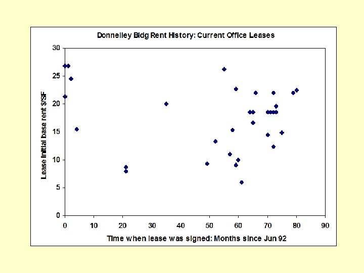
Real world example. . . The R. R. Donnelly Bldg, Chicago $280 million, 945000 SF, 50 -story Office Tower

Location: In “The Loop” (CBD) at W. Wacker Dr & N. Clark St, On the Chicago River. . .

Donnelley Bldg Pro Forma. . .

Rentt = (Rent 0)etg Ln(Rentt) = Ln(Rent 0) + tg (Rent 12/Rent 0) – 1 = e 12 g – 1 = (2. 7183)12*(-0. 00093) -1 = -1. 1% per year = Ann. rent trend, 92 -98. Infla (92 -98) = 2. 4%/yr. Real rent trend = -1. 1% - 2. 4% = -3. 5%/yr.

Section 11. 2: “Opportunity Cost of Capital” (OCC) at the Property Level or: WHERE DO DISCOUNT RATES COME FROM? . . .

Broad Answer: THE CAPITAL MARKETS That is, competing investment opportunities. (This is so, whether we are talking about IV or MV. )

IN DCF APPLICATIONS, KEEP IN MIND WHAT THE DISCOUNT RATE IS. . . Disc. Rate = Required Return = Oppty. Cost of Capital = Expected total return = rf + RP = y + g, among investors in the market today for assets similar in risk to the property in question.

NOTE: Risk is in the object not in the beholder. Property "X" has the same risk for Investor "A" as for Investor "B". Therefore, oppty cost of cap (r) is same for “A” & “B” for purposes of evaluating NPV of investment in “X” (same discount rate). Unless, say, “A” has some unique ability to alter the risk of X’s future CFs. (This is rare: be skeptical of such claims!)

Example. . . REIT A has expected total return to equity = 12%, Avg. debt int. rate = 7%, Debt/Total Asset Value Ratio = 20% What is REIT A’s (firm-level) Cost of Capital (WACC)? Ans: (0. 2)7% + (1 -0. 2)12% = 1. 4% + 9. 6% = 11%. REIT B has no debt, curr. div. yield = 6%, pays out all its earnings in dividends (share price/earnings multiple = 16. 667), avg. div. growth rate = 4%/yr. What is REIT B’s (firm-level) Cost of Capital (WACC)? [Hint: Use “Gordon Growth Model”. ] Ans: 6% + 4% = 10%.

Example (cont. ). . . Property X is a Boston Office Bldg, in a market where such bldgs sell at 8% cap rates (CF / V), with 0. 5% expected LR annual growth (in V & CF). It has initial CF = $1, 000/yr. How much can REIT A afford to pay for Prop. X (without suffering loss in share value)? Answer: Prop. X OCC = 8% + 0. 5% = 8. 5%. Prop. X Val = $1, 000 / (8. 5% - 0. 5%) = $1, 000 / 0. 08 = $12, 500, 000. Note: This is not equal to: $1, 000 / (11% - 0. 5%) = $9, 524, 000 How much can REIT B afford to pay for Prop. X (without suffering loss in share value)? Answer: Same as REIT A: Prop. X Val = $1, 000 / (8. 5% - 0. 5%) = $12, 500, 000. Note: This is not equal to: $1, 000 / (10%-4%) = $1, 000 / 6% = $16, 667, 000.

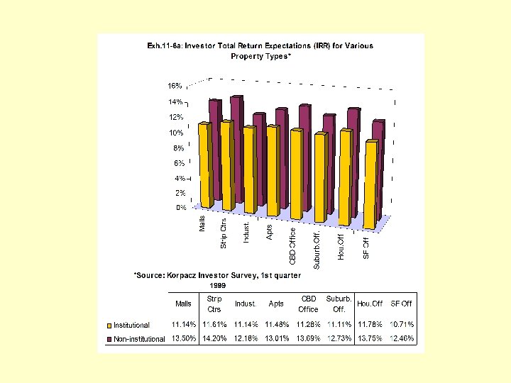
HOW DO YOU DETERMINE THE DISCOUNT RATE? . . . Usually a single ("blended") multi-year rate is OK for valuation and investment analysis ("going-in IRR"). One source of info is direct surveys of market participants. Another source is historical evidence. . .

Survey avg 200 bps > Hist. avg.

Typical per annum OCC (“going-in IRR”) rates (late 1990 s). . . For high quality ("class A", "institutional quality") income property: 10% - 12%, stated. 8% - 10%, realistic. Lower quality or more risky income property (e. g. , hotels, class B commercial, turnarounds, "mom & pops"): 12% - 15% Raw land (speculation): 15% - 30% Maybe a bit lower today.

How to "back out" implied discount rates from "cap rates" (OAR) observed from transaction prices in the property market. . . Cap rate = NOI / V CF / V = y. Therefore, from market transaction data. . . 1) Observe prices (V) 2) Observe NOI of sold properties. 3) Therefore, observe "cap rates" = NOI / V. 4) Compute: r = y + g cap rate + g.

So we can get an idea what the market's expected total return (discount rate) is for different types of properties by: observing the cap rates at which they are sold, 2. and then making reasonable assumptions about growth expectations (g). 1.

But, watch out for capital expenditures: y = CF / V cap rate = NOI / V CF = NOI - CI, (unless NOI is already net of a "reserve" for CI) CI / V 1% - 2% on avg in long run (usually). Therefore: r = y + g = (cap rate) + g - (CI/V), unless cap rate already net of CI.

Watch out for terminology: In Brealey-Myers “capitalization rate” is often used to refer to “r”, the total cost of capital (especially in corporate finance). “r” is also sometimes called the “total yield” (especially in the appraisal profession).