Relative Valuation Aswath Damodaran 1 What is relative

Relative Valuation Aswath Damodaran 1

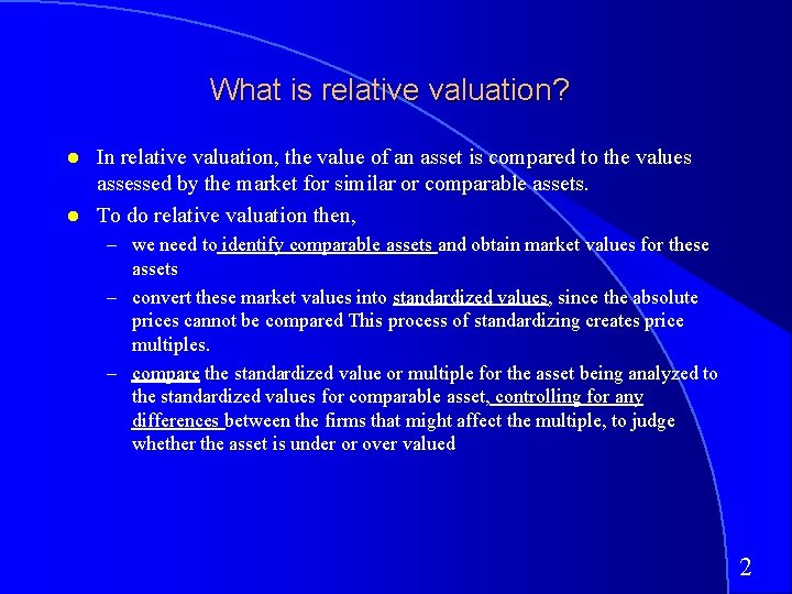
What is relative valuation? In relative valuation, the value of an asset is compared to the values assessed by the market for similar or comparable assets. To do relative valuation then, – we need to identify comparable assets and obtain market values for these assets – convert these market values into standardized values, since the absolute prices cannot be compared This process of standardizing creates price multiples. – compare the standardized value or multiple for the asset being analyzed to the standardized values for comparable asset, controlling for any differences between the firms that might affect the multiple, to judge whether the asset is under or over valued 2

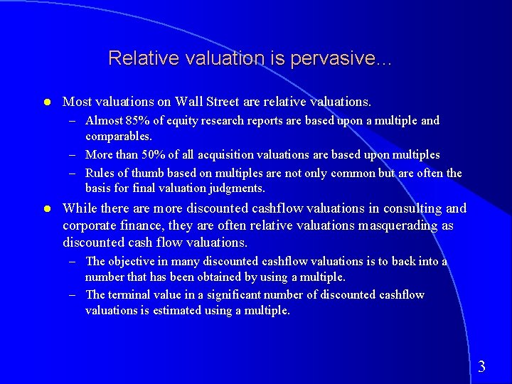
Relative valuation is pervasive… Most valuations on Wall Street are relative valuations. – Almost 85% of equity research reports are based upon a multiple and comparables. – More than 50% of all acquisition valuations are based upon multiples – Rules of thumb based on multiples are not only common but are often the basis for final valuation judgments. While there are more discounted cashflow valuations in consulting and corporate finance, they are often relative valuations masquerading as discounted cash flow valuations. – The objective in many discounted cashflow valuations is to back into a number that has been obtained by using a multiple. – The terminal value in a significant number of discounted cashflow valuations is estimated using a multiple. 3

Why relative valuation? “If you think I’m crazy, you should see the guy who lives across the hall” Jerry Seinfeld talking about Kramer in a Seinfeld episode “ A little inaccuracy sometimes saves tons of explanation” H. H. Munro “ If you are going to screw up, make sure that you have lots of company” Ex-portfolio manager 4

So, you believe only in intrinsic value? Here is why you should still care about relative value Even if you are a true believer in discounted cashflow valuation, presenting your findings on a relative valuation basis will make it more likely that your findings/recommendations will reach a receptive audience. In some cases, relative valuation can help find weak spots in discounted cash flow valuations and fix them. The problem with multiples is not in their use but in their abuse. If we can find ways to frame multiples right, we should be able to use them better. 5

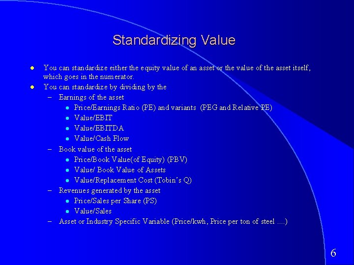
Standardizing Value You can standardize either the equity value of an asset or the value of the asset itself, which goes in the numerator. You can standardize by dividing by the – Earnings of the asset Price/Earnings Ratio (PE) and variants (PEG and Relative PE) Value/EBITDA Value/Cash Flow – Book value of the asset Price/Book Value(of Equity) (PBV) Value/ Book Value of Assets Value/Replacement Cost (Tobin’s Q) – Revenues generated by the asset Price/Sales per Share (PS) Value/Sales – Asset or Industry Specific Variable (Price/kwh, Price per ton of steel. . ) 6

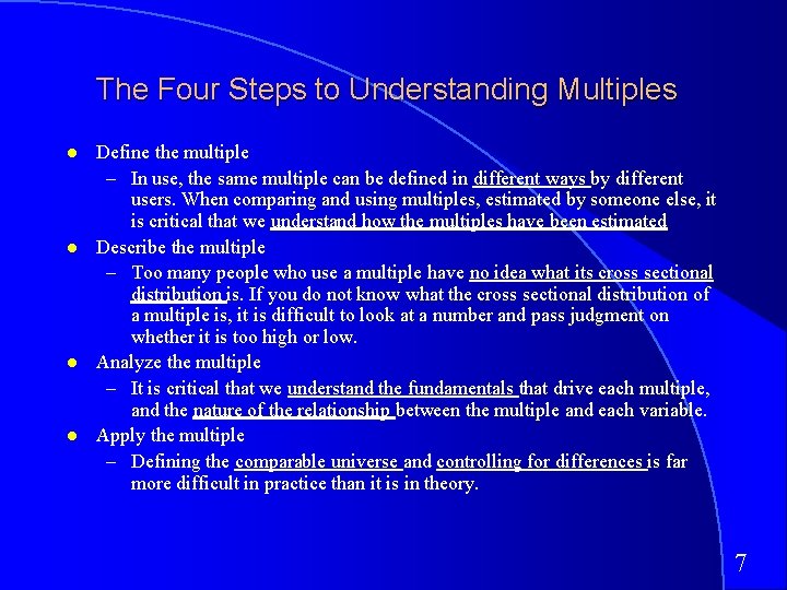
The Four Steps to Understanding Multiples Define the multiple – In use, the same multiple can be defined in different ways by different users. When comparing and using multiples, estimated by someone else, it is critical that we understand how the multiples have been estimated Describe the multiple – Too many people who use a multiple have no idea what its cross sectional distribution is. If you do not know what the cross sectional distribution of a multiple is, it is difficult to look at a number and pass judgment on whether it is too high or low. Analyze the multiple – It is critical that we understand the fundamentals that drive each multiple, and the nature of the relationship between the multiple and each variable. Apply the multiple – Defining the comparable universe and controlling for differences is far more difficult in practice than it is in theory. 7

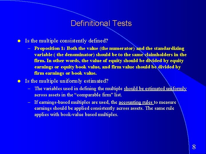
Definitional Tests Is the multiple consistently defined? – Proposition 1: Both the value (the numerator) and the standardizing variable ( the denominator) should be to the same claimholders in the firm. In other words, the value of equity should be divided by equity earnings or equity book value, and firm value should be divided by firm earnings or book value. Is the multiple uniformly estimated? – The variables used in defining the multiple should be estimated uniformly across assets in the “comparable firm” list. – If earnings-based multiples are used, the accounting rules to measure earnings should be applied consistently across assets. The same rule applies with book-value based multiples. 8

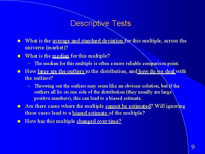
Descriptive Tests What is the average and standard deviation for this multiple, across the universe (market)? What is the median for this multiple? – The median for this multiple is often a more reliable comparison point. How large are the outliers to the distribution, and how do we deal with the outliers? – Throwing out the outliers may seem like an obvious solution, but if the outliers all lie on one side of the distribution (they usually are large positive numbers), this can lead to a biased estimate. Are there cases where the multiple cannot be estimated? Will ignoring these cases lead to a biased estimate of the multiple? How has this multiple changed over time? 9

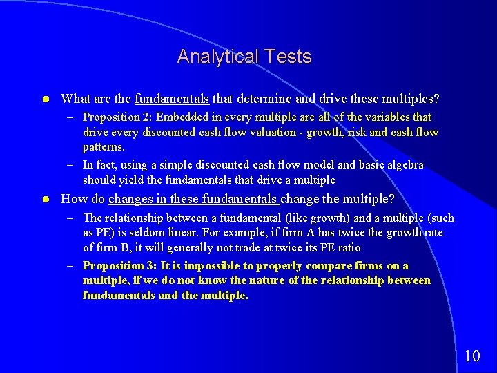
Analytical Tests What are the fundamentals that determine and drive these multiples? – Proposition 2: Embedded in every multiple are all of the variables that drive every discounted cash flow valuation - growth, risk and cash flow patterns. – In fact, using a simple discounted cash flow model and basic algebra should yield the fundamentals that drive a multiple How do changes in these fundamentals change the multiple? – The relationship between a fundamental (like growth) and a multiple (such as PE) is seldom linear. For example, if firm A has twice the growth rate of firm B, it will generally not trade at twice its PE ratio – Proposition 3: It is impossible to properly compare firms on a multiple, if we do not know the nature of the relationship between fundamentals and the multiple. 10

Application Tests Given the firm that we are valuing, what is a “comparable” firm? – While traditional analysis is built on the premise that firms in the same sector are comparable firms, valuation theory would suggest that a comparable firm is one which is similar to the one being analyzed in terms of fundamentals. – Proposition 4: There is no reason why a firm cannot be compared with another firm in a very different business, if the two firms have the same risk, growth and cash flow characteristics. Given the comparable firms, how do we adjust for differences across firms on the fundamentals? – Proposition 5: It is impossible to find an exactly identical firm to the one you are valuing. 11

Price Earnings Ratio: Definition PE = Market Price per Share / Earnings per Share There a number of variants on the basic PE ratio in use. They are based upon how the price and the earnings are defined. Price: is usually the current price is sometimes the average price for the year EPS: earnings per share in most recent financial year earnings per share in trailing 12 months (Trailing PE) forecasted earnings per share next year (Forward PE) forecasted earnings per share in future year 12

Looking at the distribution… 13

PE: Deciphering the Distribution 14

Comparing PE Ratios: US, Europe, Japan and Emerging Markets - January 2005 Median PE Japan = 23. 45 US = 23. 21 Europe = 18. 79 Em. Mkts = 16. 18 15

PE Ratios in Brazil - January 2006 16

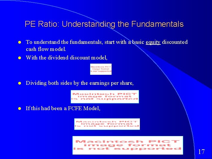
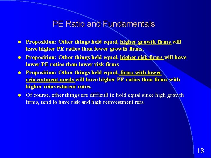
PE Ratio: Understanding the Fundamentals To understand the fundamentals, start with a basic equity discounted cash flow model. With the dividend discount model, Dividing both sides by the earnings per share, If this had been a FCFE Model, 17

PE Ratio and Fundamentals Proposition: Other things held equal, higher growth firms will have higher PE ratios than lower growth firms. Proposition: Other things held equal, higher risk firms will have lower PE ratios than lower risk firms Proposition: Other things held equal, firms with lower reinvestment needs will have higher PE ratios than firms with higher reinvestment rates. Of course, other things are difficult to hold equal since high growth firms, tend to have risk and high reinvestment rats. 18

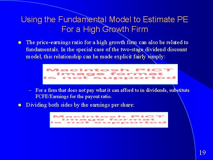
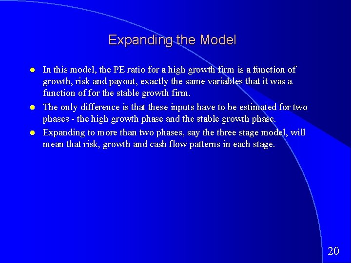
Using the Fundamental Model to Estimate PE For a High Growth Firm The price-earnings ratio for a high growth firm can also be related to fundamentals. In the special case of the two-stage dividend discount model, this relationship can be made explicit fairly simply: – For a firm that does not pay what it can afford to in dividends, substitute FCFE/Earnings for the payout ratio. Dividing both sides by the earnings per share: 19

Expanding the Model In this model, the PE ratio for a high growth firm is a function of growth, risk and payout, exactly the same variables that it was a function of for the stable growth firm. The only difference is that these inputs have to be estimated for two phases - the high growth phase and the stable growth phase. Expanding to more than two phases, say the three stage model, will mean that risk, growth and cash flow patterns in each stage. 20

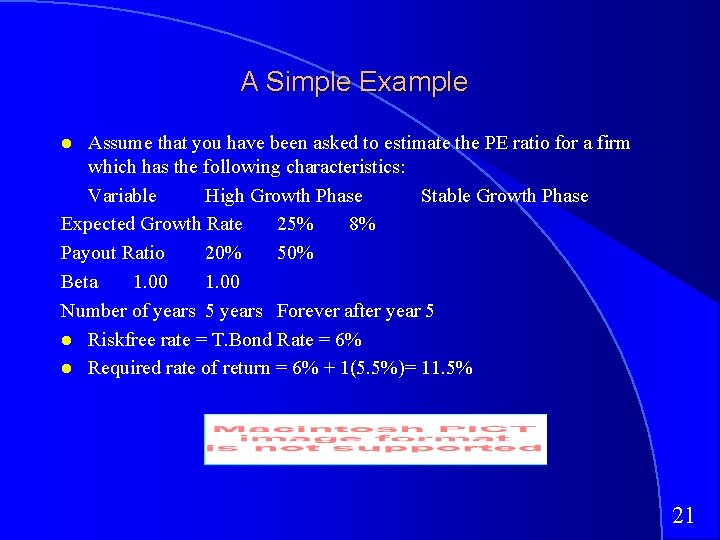
A Simple Example Assume that you have been asked to estimate the PE ratio for a firm which has the following characteristics: Variable High Growth Phase Stable Growth Phase Expected Growth Rate 25% 8% Payout Ratio 20% 50% Beta 1. 00 Number of years 5 years Forever after year 5 Riskfree rate = T. Bond Rate = 6% Required rate of return = 6% + 1(5. 5%)= 11. 5% 21

PE and Growth: Firm grows at x% for 5 years, 8% thereafter 22

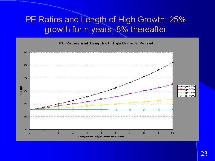
PE Ratios and Length of High Growth: 25% growth for n years; 8% thereafter 23

PE and Risk: Effects of Changing Betas on PE Ratio: Firm with x% growth for 5 years; 8% thereafter 24

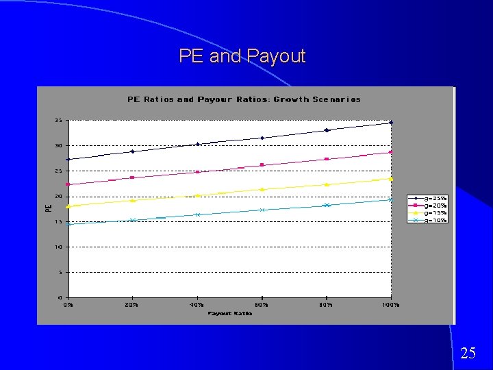
PE and Payout 25

I. Comparisons of PE across time: PE Ratio for the S&P 500 26

Is low (high) PE cheap (expensive)? A market strategist argues that stocks are over priced because the PE ratio today is too high relative to the average PE ratio across time. Do you agree? q Yes q No If you do not agree, what factors might explain the higher PE ratio today? 27

E/P Ratios , T. Bond Rates and Term Structure 28

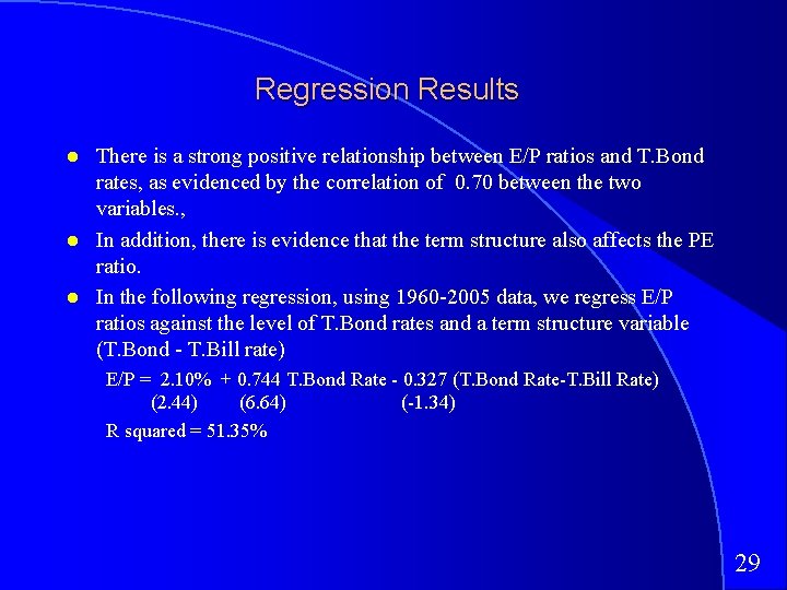
Regression Results There is a strong positive relationship between E/P ratios and T. Bond rates, as evidenced by the correlation of 0. 70 between the two variables. , In addition, there is evidence that the term structure also affects the PE ratio. In the following regression, using 1960 -2005 data, we regress E/P ratios against the level of T. Bond rates and a term structure variable (T. Bond - T. Bill rate) E/P = 2. 10% + 0. 744 T. Bond Rate - 0. 327 (T. Bond Rate-T. Bill Rate) (2. 44) (6. 64) (-1. 34) R squared = 51. 35% 29

II. Comparing PE Ratios across a Sector 30

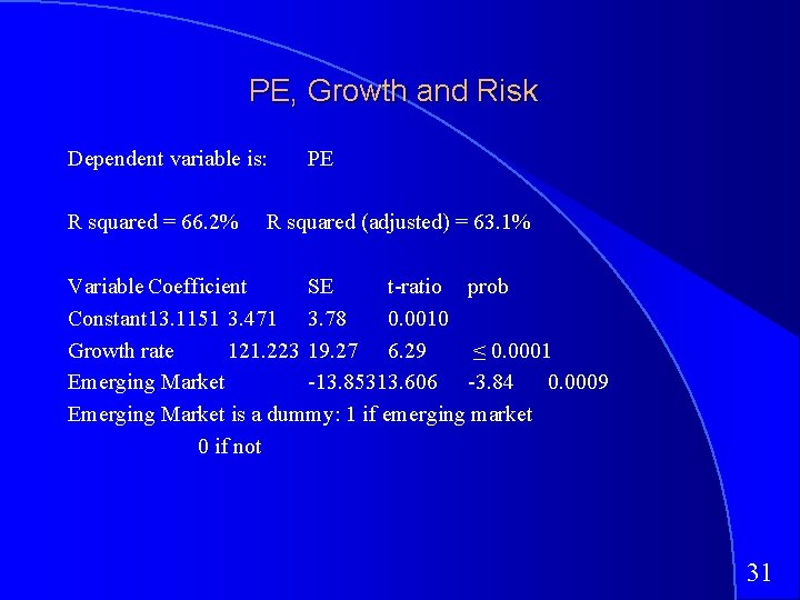
PE, Growth and Risk Dependent variable is: R squared = 66. 2% PE R squared (adjusted) = 63. 1% Variable Coefficient SE t-ratio prob Constant 13. 1151 3. 471 3. 78 0. 0010 Growth rate 121. 223 19. 27 6. 29 ≤ 0. 0001 Emerging Market -13. 85313. 606 -3. 84 0. 0009 Emerging Market is a dummy: 1 if emerging market 0 if not 31

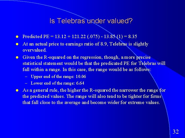
Is Telebras under valued? Predicted PE = 13. 12 + 121. 22 (. 075) - 13. 85 (1) = 8. 35 At an actual price to earnings ratio of 8. 9, Telebras is slightly overvalued. Given the R-squared on the regression, though, a more precise statistical statement would be that the predicated PE for Telebras will fall within a range. In this case, the range would be as follows: – Upper end of the range: 10. 06 – Lower end of the range: 6. 64 As a general rule, the higher the R-squared the narrower the range for the predicted values. The range will also tend to be tighter for firms that fall close to the average and become wider for extreme values. 32

Using the entire crosssection: A regression approach In contrast to the 'comparable firm' approach, the information in the entire cross-section of firms can be used to predict PE ratios. The simplest way of summarizing this information is with a multiple regression, with the PE ratio as the dependent variable, and proxies for risk, growth and payout forming the independent variables. 33

PE versus Growth 34

PE Ratio: Standard Regression for US stocks January 2006 35

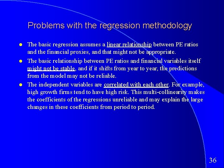
Problems with the regression methodology The basic regression assumes a linear relationship between PE ratios and the financial proxies, and that might not be appropriate. The basic relationship between PE ratios and financial variables itself might not be stable, and if it shifts from year to year, the predictions from the model may not be reliable. The independent variables are correlated with each other. For example, high growth firms tend to have high risk. This multi-collinearity makes the coefficients of the regressions unreliable and may explain the large changes in these coefficients from period to period. 36

The Multicollinearity Problem 37

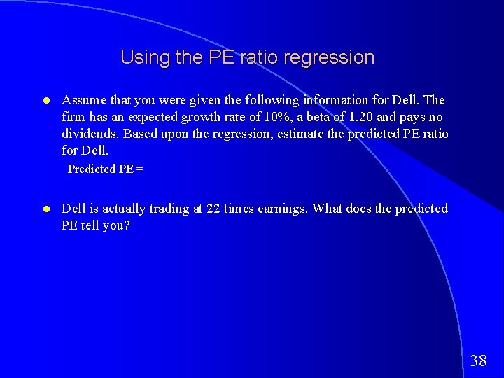
Using the PE ratio regression Assume that you were given the following information for Dell. The firm has an expected growth rate of 10%, a beta of 1. 20 and pays no dividends. Based upon the regression, estimate the predicted PE ratio for Dell. Predicted PE = Dell is actually trading at 22 times earnings. What does the predicted PE tell you? 38

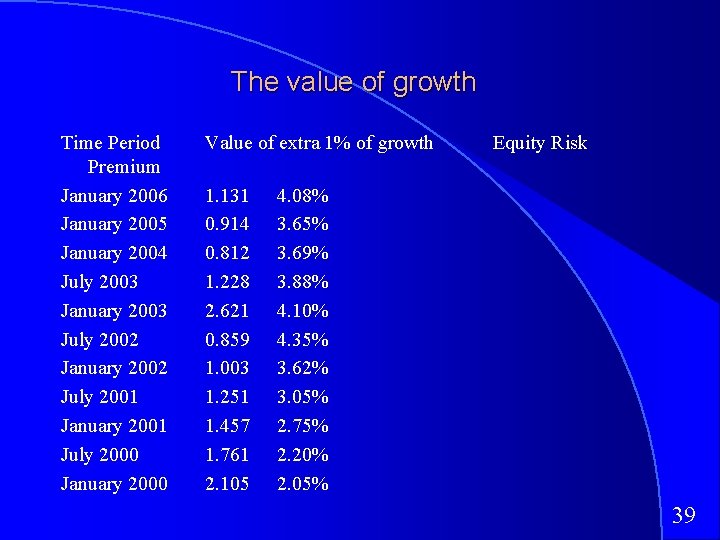
The value of growth Time Period Premium January 2006 January 2005 January 2004 July 2003 January 2003 July 2002 January 2002 July 2001 January 2001 July 2000 January 2000 Value of extra 1% of growth 1. 131 0. 914 0. 812 1. 228 2. 621 0. 859 1. 003 1. 251 1. 457 1. 761 2. 105 Equity Risk 4. 08% 3. 65% 3. 69% 3. 88% 4. 10% 4. 35% 3. 62% 3. 05% 2. 75% 2. 20% 2. 05% 39

Brazil: Cross Sectional Regression January 2006 40

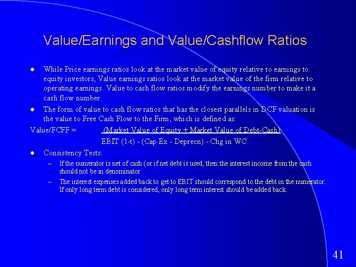
Value/Earnings and Value/Cashflow Ratios While Price earnings ratios look at the market value of equity relative to earnings to equity investors, Value earnings ratios look at the market value of the firm relative to operating earnings. Value to cash flow ratios modify the earnings number to make it a cash flow number. The form of value to cash flow ratios that has the closest parallels in DCF valuation is the value to Free Cash Flow to the Firm, which is defined as: Value/FCFF = (Market Value of Equity + Market Value of Debt-Cash) EBIT (1 -t) - (Cap Ex - Deprecn) - Chg in WC Consistency Tests: – – If the numerator is net of cash (or if net debt is used, then the interest income from the cash should not be in denominator The interest expenses added back to get to EBIT should correspond to the debt in the numerator. If only long term debt is considered, only long term interest should be added back. 41

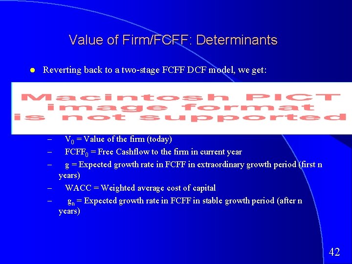
Value of Firm/FCFF: Determinants Reverting back to a two-stage FCFF DCF model, we get: – – – V 0 = Value of the firm (today) FCFF 0 = Free Cashflow to the firm in current year g = Expected growth rate in FCFF in extraordinary growth period (first n years) – WACC = Weighted average cost of capital – gn = Expected growth rate in FCFF in stable growth period (after n years) 42

Value Multiples Dividing both sides by the FCFF yields, The value/FCFF multiples is a function of – the cost of capital – the expected growth 43

Value/FCFF Multiples and the Alternatives Assume that you have computed the value of a firm, using discounted cash flow models. Rank the following multiples in the order of magnitude from lowest to highest? Value/EBIT(1 -t) Value/FCFF Value/EBITDA What assumption(s) would you need to make for the Value/EBIT(1 -t) ratio to be equal to the Value/FCFF multiple? 44

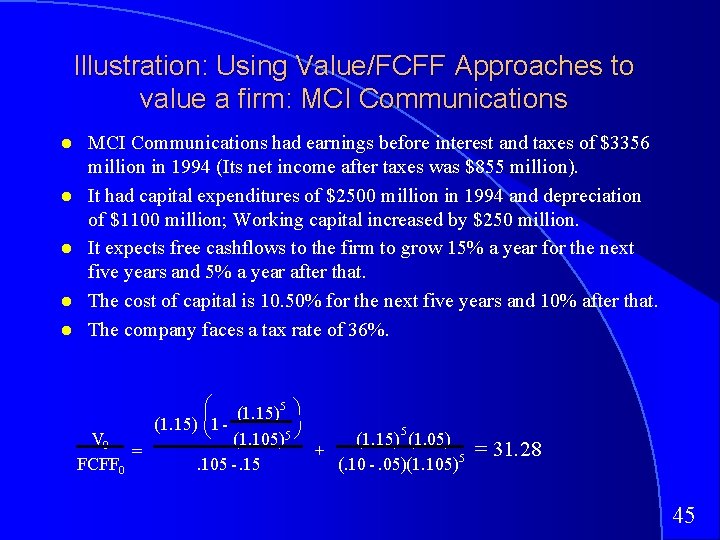
Illustration: Using Value/FCFF Approaches to value a firm: MCI Communications had earnings before interest and taxes of $3356 million in 1994 (Its net income after taxes was $855 million). It had capital expenditures of $2500 million in 1994 and depreciation of $1100 million; Working capital increased by $250 million. It expects free cashflows to the firm to grow 15% a year for the next five years and 5% a year after that. The cost of capital is 10. 50% for the next five years and 10% after that. The company faces a tax rate of 36%. V 0 = FCFF 0 æç (1. 15)5 ö (1. 15) è 1(1. 105)5 ø. 105 -. 15 5 (1. 15) (1. 05) = 31. 28 + 5 (. 10 -. 05)(1. 105) 45

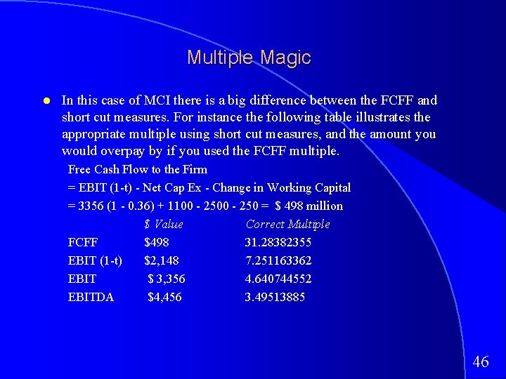
Multiple Magic In this case of MCI there is a big difference between the FCFF and short cut measures. For instance the following table illustrates the appropriate multiple using short cut measures, and the amount you would overpay by if you used the FCFF multiple. Free Cash Flow to the Firm = EBIT (1 -t) - Net Cap Ex - Change in Working Capital = 3356 (1 - 0. 36) + 1100 - 250 = $ 498 million $ Value Correct Multiple FCFF $498 31. 28382355 EBIT (1 -t) $2, 148 7. 251163362 EBIT $ 3, 356 4. 640744552 EBITDA $4, 456 3. 49513885 46

Reasons for Increased Use of Value/EBITDA 1. The multiple can be computed even for firms that are reporting net losses, since earnings before interest, taxes and depreciation are usually positive. 2. For firms in certain industries, such as cellular, which require a substantial investment in infrastructure and long gestation periods, this multiple seems to be more appropriate than the price/earnings ratio. 3. In leveraged buyouts, where the key factor is cash generated by the firm prior to all discretionary expenditures, the EBITDA is the measure of cash flows from operations that can be used to support debt payment at least in the short term. 4. By looking at cashflows prior to capital expenditures, it may provide a better estimate of “optimal value”, especially if the capital expenditures are unwise or earn substandard returns. 5. By looking at the value of the firm and cashflows to the firm it allows for comparisons across firms with different financial leverage. 47

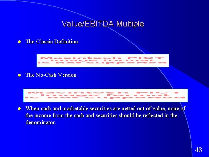
Value/EBITDA Multiple The Classic Definition The No-Cash Version When cash and marketable securities are netted out of value, none of the income from the cash and securities should be reflected in the denominator. 48

Enterprise Value/EBITDA Distribution - US 49

EV/EBITDA Multiple: Brazil in January 2006 50

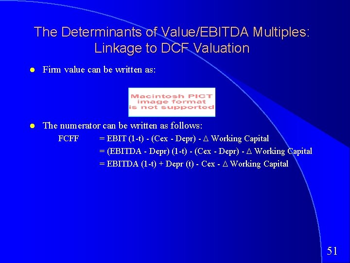
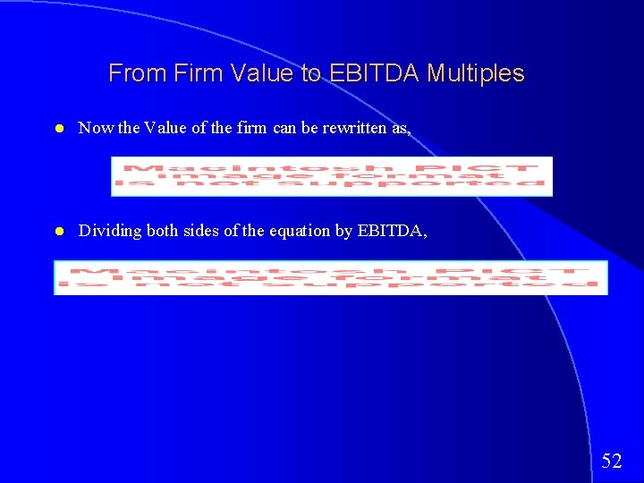
The Determinants of Value/EBITDA Multiples: Linkage to DCF Valuation Firm value can be written as: The numerator can be written as follows: FCFF = EBIT (1 -t) - (Cex - Depr) - Working Capital = (EBITDA - Depr) (1 -t) - (Cex - Depr) - Working Capital = EBITDA (1 -t) + Depr (t) - Cex - Working Capital 51

From Firm Value to EBITDA Multiples Now the Value of the firm can be rewritten as, Dividing both sides of the equation by EBITDA, 52

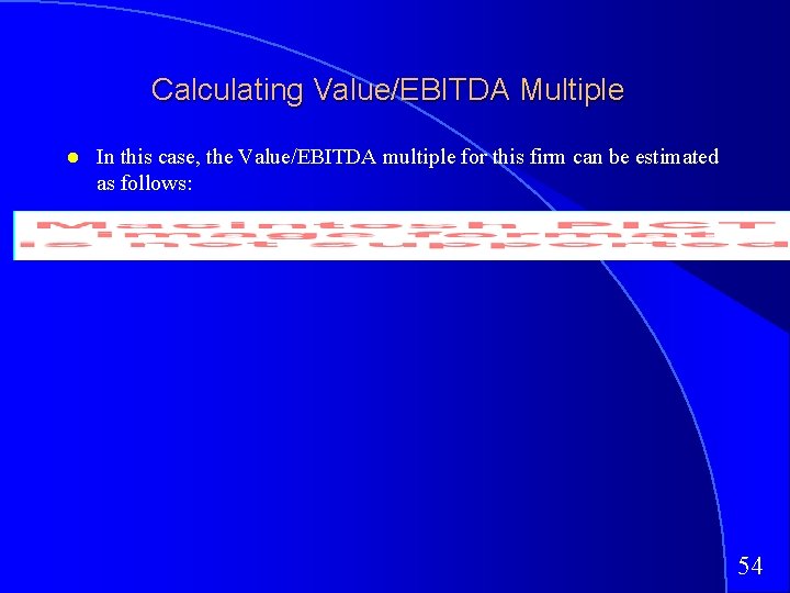
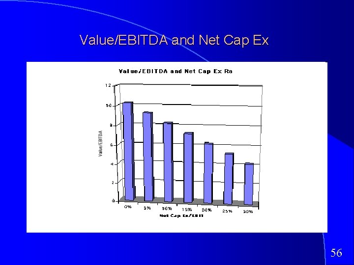
A Simple Example Consider a firm with the following characteristics: – – – Tax Rate = 36% Capital Expenditures/EBITDA = 30% Depreciation/EBITDA = 20% Cost of Capital = 10% The firm has no working capital requirements The firm is in stable growth and is expected to grow 5% a year forever. 53

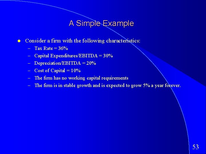
Calculating Value/EBITDA Multiple In this case, the Value/EBITDA multiple for this firm can be estimated as follows: 54

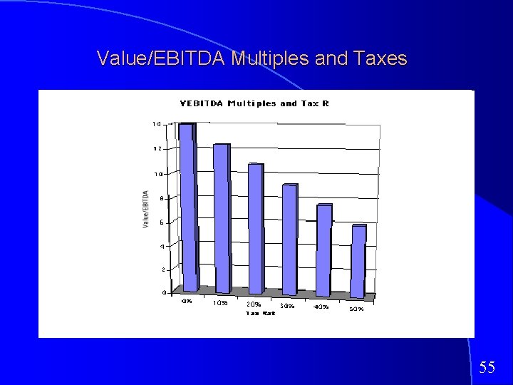
Value/EBITDA Multiples and Taxes 55

Value/EBITDA and Net Cap Ex 56

Value/EBITDA Multiples and Return on Capital 57

Value/EBITDA Multiple: Trucking Companies 58

A Test on EBITDA Ryder System looks very cheap on a Value/EBITDA multiple basis, relative to the rest of the sector. What explanation (other than misvaluation) might there be for this difference? 59

US Market: Cross Sectional Regression January 2006 60

Price-Book Value Ratio: Definition The price/book value ratio is the ratio of the market value of equity to the book value of equity, i. e. , the measure of shareholders’ equity in the balance sheet. Price/Book Value = Market Value of Equity Book Value of Equity Consistency Tests: – If the market value of equity refers to the market value of equity of common stock outstanding, the book value of common equity should be used in the denominator. – If there is more that one class of common stock outstanding, the market values of all classes (even the non-traded classes) needs to be factored in. 61

Book Value Multiples: US stocks 62

Book Value Multiples: Brazil 63

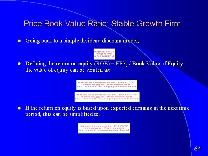
Price Book Value Ratio: Stable Growth Firm Going back to a simple dividend discount model, Defining the return on equity (ROE) = EPS 0 / Book Value of Equity, the value of equity can be written as: If the return on equity is based upon expected earnings in the next time period, this can be simplified to, 64

PBV/ROE: European Banks 65

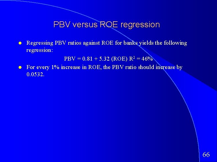
PBV versus ROE regression Regressing PBV ratios against ROE for banks yields the following regression: PBV = 0. 81 + 5. 32 (ROE) R 2 = 46% For every 1% increase in ROE, the PBV ratio should increase by 0. 0532. 66

Under and Over Valued Banks? 67

Looking for undervalued securities - PBV Ratios and ROE : The Valuation Matrix 68

Price to Book vs ROE: US companies in January 2005 69

PBV Matrix: Telecom Companies 70

PBV, ROE and Risk: Large Cap US firms 71

PBV versus ROE: Brazilian companies in January 2006 72

IBM: The Rise and Fall and Rise Again 73

PBV Ratio Regression: US January 2006 74

PBV Regression: Brazil in January 2006 75

Price Sales Ratio: Definition The price/sales ratio is the ratio of the market value of equity to the sales. Price/ Sales= Market Value of Equity Total Revenues Consistency Tests – The price/sales ratio is internally inconsistent, since the market value of equity is divided by the total revenues of the firm. 76

Revenue Multiples: US stocks 77

Revenue Multiples: Brazil 78

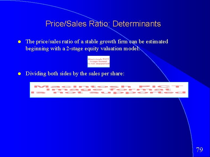
Price/Sales Ratio: Determinants The price/sales ratio of a stable growth firm can be estimated beginning with a 2 -stage equity valuation model: Dividing both sides by the sales per share: 79

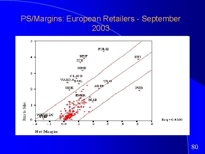
PS/Margins: European Retailers - September 2003 80

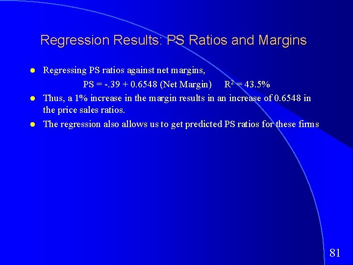
Regression Results: PS Ratios and Margins Regressing PS ratios against net margins, PS = -. 39 + 0. 6548 (Net Margin) R 2 = 43. 5% Thus, a 1% increase in the margin results in an increase of 0. 6548 in the price sales ratios. The regression also allows us to get predicted PS ratios for these firms 81

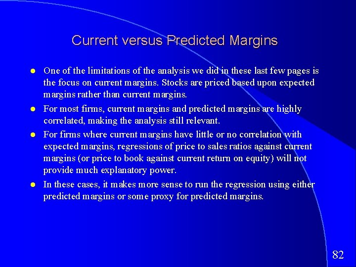
Current versus Predicted Margins One of the limitations of the analysis we did in these last few pages is the focus on current margins. Stocks are priced based upon expected margins rather than current margins. For most firms, current margins and predicted margins are highly correlated, making the analysis still relevant. For firms where current margins have little or no correlation with expected margins, regressions of price to sales ratios against current margins (or price to book against current return on equity) will not provide much explanatory power. In these cases, it makes more sense to run the regression using either predicted margins or some proxy for predicted margins. 82

A Case Study: The Internet Stocks 83

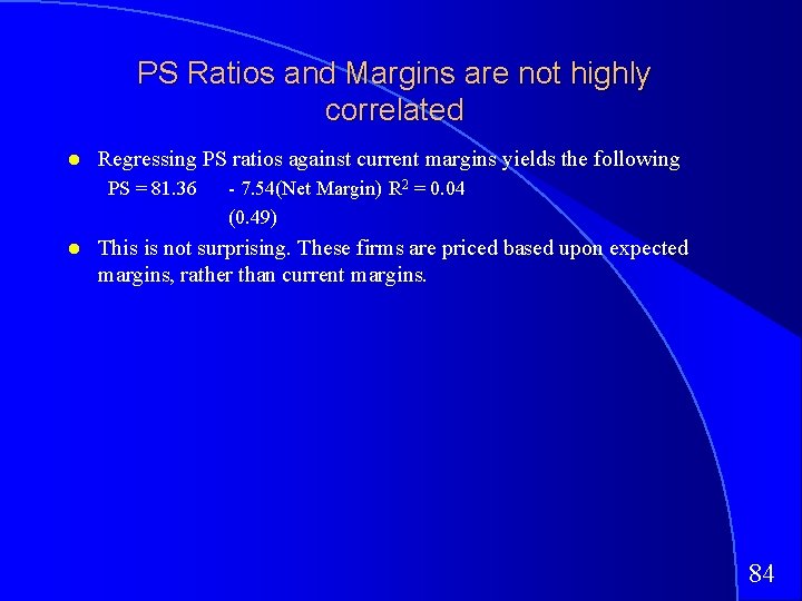
PS Ratios and Margins are not highly correlated Regressing PS ratios against current margins yields the following PS = 81. 36 - 7. 54(Net Margin) R 2 = 0. 04 (0. 49) This is not surprising. These firms are priced based upon expected margins, rather than current margins. 84

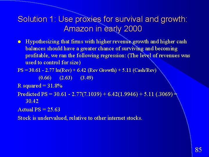
Solution 1: Use proxies for survival and growth: Amazon in early 2000 Hypothesizing that firms with higher revenue growth and higher cash balances should have a greater chance of surviving and becoming profitable, we ran the following regression: (The level of revenues was used to control for size) PS = 30. 61 - 2. 77 ln(Rev) + 6. 42 (Rev Growth) + 5. 11 (Cash/Rev) (0. 66) (2. 63) (3. 49) R squared = 31. 8% Predicted PS = 30. 61 - 2. 77(7. 1039) + 6. 42(1. 9946) + 5. 11 (. 3069) = 30. 42 Actual PS = 25. 63 Stock is undervalued, relative to other internet stocks. 85

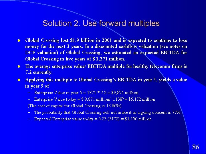
Solution 2: Use forward multiples Global Crossing lost $1. 9 billion in 2001 and is expected to continue to lose money for the next 3 years. In a discounted cashflow valuation (see notes on DCF valuation) of Global Crossing, we estimated an expected EBITDA for Global Crossing in five years of $ 1, 371 million. The average enterprise value/ EBITDA multiple for healthy telecomm firms is 7. 2 currently. Applying this multiple to Global Crossing’s EBITDA in year 5, yields a value in year 5 of – Enterprise Value in year 5 = 1371 * 7. 2 = $9, 871 million – Enterprise Value today = $ 9, 871 million/ 1. 1385 = $5, 172 million (The cost of capital for Global Crossing is 13. 80%) – The probability that Global Crossing will not make it as a going concern is 77%. – Expected Enterprise value today = 0. 23 (5172) = $1, 190 million 86

PS Regression: United States - January 2006 87

EV/Sales Regression: Brazil in January 2006 88

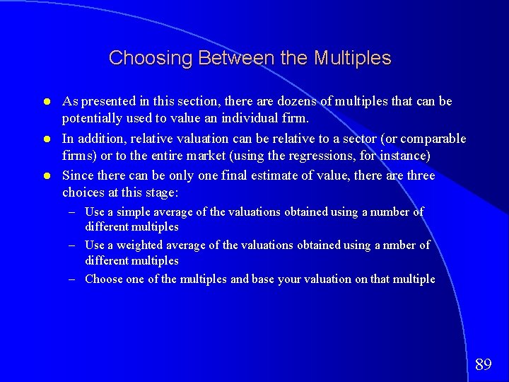
Choosing Between the Multiples As presented in this section, there are dozens of multiples that can be potentially used to value an individual firm. In addition, relative valuation can be relative to a sector (or comparable firms) or to the entire market (using the regressions, for instance) Since there can be only one final estimate of value, there are three choices at this stage: – Use a simple average of the valuations obtained using a number of different multiples – Use a weighted average of the valuations obtained using a nmber of different multiples – Choose one of the multiples and base your valuation on that multiple 89

Picking one Multiple This is usually the best way to approach this issue. While a range of values can be obtained from a number of multiples, the “best estimate” value is obtained using one multiple. The multiple that is used can be chosen in one of two ways: – Use the multiple that best fits your objective. Thus, if you want the company to be undervalued, you pick the multiple that yields the highest value. – Use the multiple that has the highest R-squared in the sector when regressed against fundamentals. Thus, if you have tried PE, PBV, PS, etc. and run regressions of these multiples against fundamentals, use the multiple that works best at explaining differences across firms in that sector. – Use the multiple that seems to make the most sense for that sector, given how value is measured and created. 90

A More Intuitive Approach Managers in every sector tend to focus on specific variables when analyzing strategy and performance. The multiple used will generally reflect this focus. Consider three examples. – In retailing: The focus is usually on same store sales (turnover) and profit margins. Not surprisingly, the revenue multiple is most common in this sector. – In financial services: The emphasis is usually on return on equity. Book Equity is often viewed as a scarce resource, since capital ratios are based upon it. Price to book ratios dominate. – In technology: Growth is usually the dominant theme. PEG ratios were invented in this sector. 91

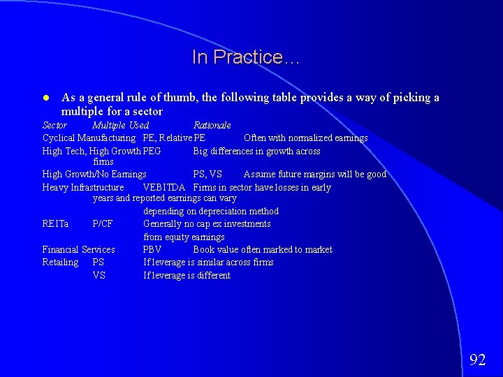
In Practice… As a general rule of thumb, the following table provides a way of picking a multiple for a sector Sector Multiple Used Rationale Cyclical Manufacturing PE, Relative PE Often with normalized earnings High Tech, High Growth PEG Big differences in growth across firms High Growth/No Earnings PS, VS Assume future margins will be good Heavy Infrastructure VEBITDA Firms in sector have losses in early years and reported earnings can vary depending on depreciation method REITa P/CF Generally no cap ex investments from equity earnings Financial Services PBV Book value often marked to market Retailing PS If leverage is similar across firms VS If leverage is different 92

Reviewing: The Four Steps to Understanding Multiples Define the multiple – Check for consistency – Make sure that they are estimated uniformly Describe the multiple – Multiples have skewed distributions: The averages are seldom good indicators of typical multiples – Check for bias, if the multiple cannot be estimated Analyze the multiple – Identify the companion variable that drives the multiple – Examine the nature of the relationship Apply the multiple 93

Real Options: Fact and Fantasy Aswath Damodaran 94

Underlying Theme: Searching for an Elusive Premium Traditional discounted cashflow models under estimate the value of investments, where there are options embedded in the investments to – Delay or defer making the investment (delay) – Adjust or alter production schedules as price changes (flexibility) – Expand into new markets or products at later stages in the process, based upon observing favorable outcomes at the early stages (expansion) – Stop production or abandon investments if the outcomes are unfavorable at early stages (abandonment) Put another way, real option advocates believe that you should be paying a premium on discounted cashflow value estimates. 95

A Real Option Premium In the last few years, there are some who have argued that discounted cashflow valuations under valued some companies and that a real option premium should be tacked on to DCF valuations. To understanding its moorings, compare the two trees below: A bad investment…………………. . Becomes a good one. . 1. Learn at relatively low cost 2. Make better decisions based on learning 96

Three Basic Questions When is there a real option embedded in a decision or an asset? When does that real option have significant economic value? Can that value be estimated using an option pricing model? 97

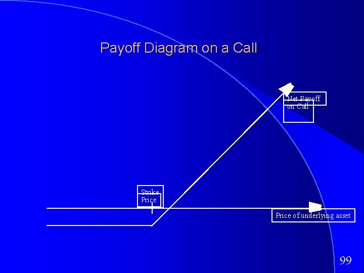
When is there an option embedded in an action? An option provides the holder with the right to buy or sell a specified quantity of an underlying asset at a fixed price (called a strike price or an exercise price) at or before the expiration date of the option. There has to be a clearly defined underlying asset whose value changes over time in unpredictable ways. The payoffs on this asset (real option) have to be contingent on an specified event occurring within a finite period. 98

Payoff Diagram on a Call Net Payoff on Call Strike Price of underlying asset 99

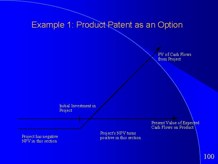
Example 1: Product Patent as an Option PV of Cash Flows from Project Initial Investment in Project Present Value of Expected Cash Flows on Product Project has negative NPV in this section Project's NPV turns positive in this section 100

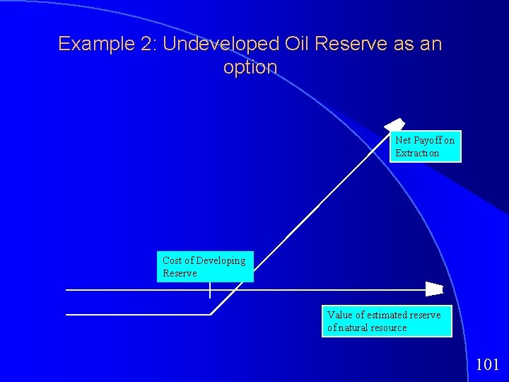
Example 2: Undeveloped Oil Reserve as an option Net Payoff on Extraction Cost of Developing Reserve Value of estimated reserve of natural resource 101

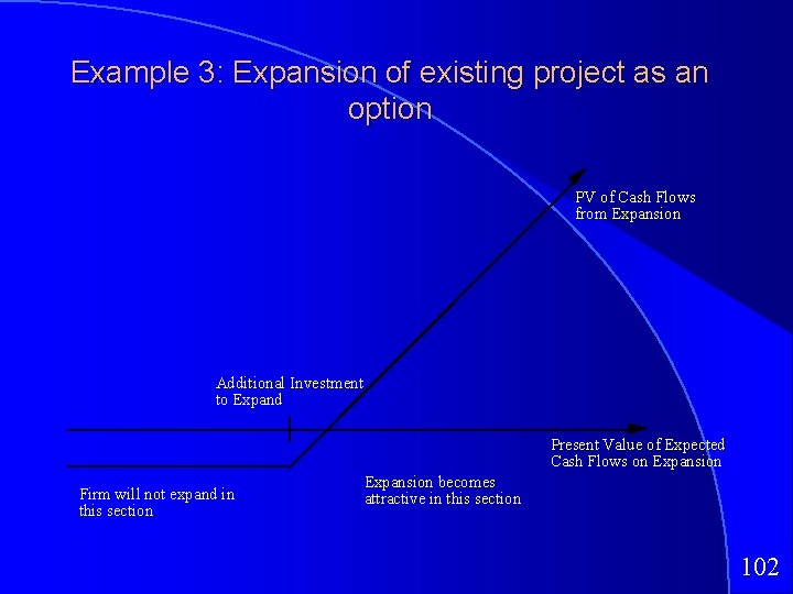
Example 3: Expansion of existing project as an option PV of Cash Flows from Expansion Additional Investment to Expand Present Value of Expected Cash Flows on Expansion Firm will not expand in this section Expansion becomes attractive in this section 102

When does the option have significant economic value? For an option to have significant economic value, there has to be a restriction on competition in the event of the contingency. In a perfectly competitive product market, no contingency, no matter how positive, will generate positive net present value. At the limit, real options are most valuable when you have exclusivity you and only you can take advantage of the contingency. They become less valuable as the barriers to competition become less steep. 103

Exclusivity: Putting Real Options to the Test Product Options: Patent on a drug – Patents restrict competitors from developing similar products – Patents do not restrict competitors from developing other products to treat the same disease. Natural Resource options: An undeveloped oil reserve or gold mine. – Natural resource reserves are limited. – It takes time and resources to develop new reserves Growth Options: Expansion into a new product or market – Barriers may range from strong (exclusive licenses granted by the government - as in telecom businesses) to weaker (brand name, knowledge of the market) to weakest (first mover). 104

Determinants of option value Variables Relating to Underlying Asset – Value of Underlying Asset; as this value increases, the right to buy at a fixed price (calls) will become more valuable and the right to sell at a fixed price (puts) will become less valuable. – Variance in that value; as the variance increases, both calls and puts will become more valuable because all options have limited downside and depend upon price volatility for upside. – Expected dividends on the asset, which are likely to reduce the price appreciation component of the asset, reducing the value of calls and increasing the value of puts. Variables Relating to Option – Strike Price of Options; the right to buy (sell) at a fixed price becomes more (less) valuable at a lower price. – Life of the Option; both calls and puts benefit from a longer life. Level of Interest Rates; as rates increase, the right to buy (sell) at a fixed price in the future becomes more (less) valuable. 105

The Building Blocks for Option Pricing Models: Arbitrage and Replication The objective in creating a replicating portfolio is to use a combination of riskfree borrowing/lending and the underlying asset to create the same cashflows as the option being valued. – Call = Borrowing + Buying of the Underlying Stock – Put = Selling Short on Underlying Asset + Lending – The number of shares bought or sold is called the option delta. The principles of arbitrage then apply, and the value of the option has to be equal to the value of the replicating portfolio. 106

The Binomial Option Pricing Model 107

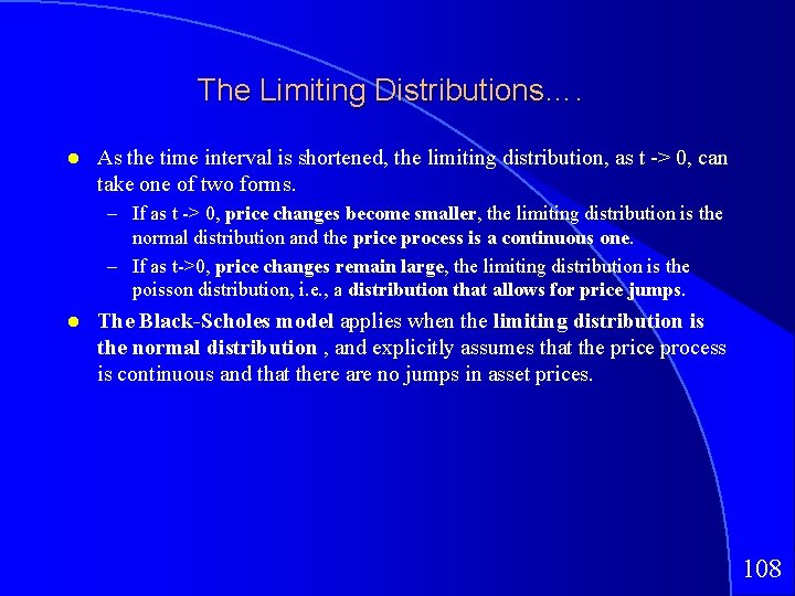
The Limiting Distributions…. As the time interval is shortened, the limiting distribution, as t -> 0, can take one of two forms. – If as t -> 0, price changes become smaller, the limiting distribution is the normal distribution and the price process is a continuous one. – If as t->0, price changes remain large, the limiting distribution is the poisson distribution, i. e. , a distribution that allows for price jumps. The Black-Scholes model applies when the limiting distribution is the normal distribution , and explicitly assumes that the price process is continuous and that there are no jumps in asset prices. 108

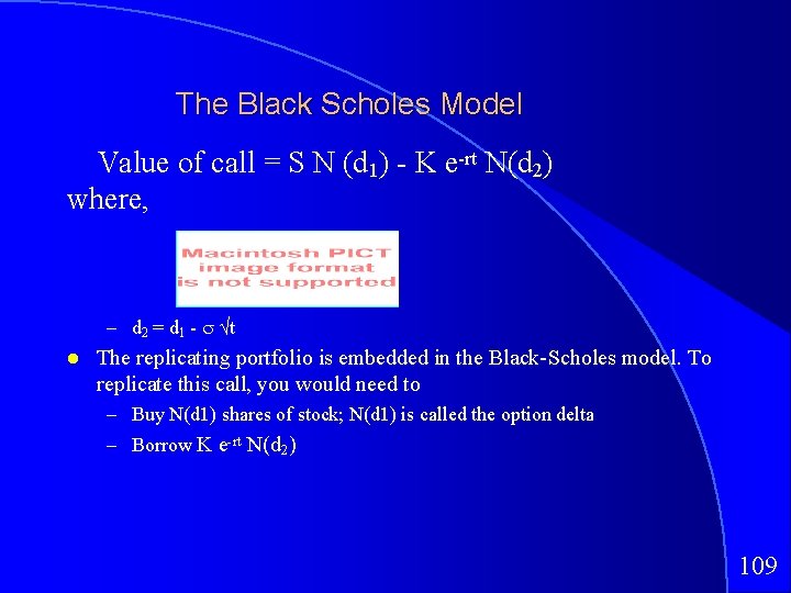
The Black Scholes Model Value of call = S N (d 1) - K e-rt N(d 2) where, – d 2 = d 1 - √t The replicating portfolio is embedded in the Black-Scholes model. To replicate this call, you would need to – Buy N(d 1) shares of stock; N(d 1) is called the option delta – Borrow K e-rt N(d 2) 109

The Normal Distribution 110

When can you use option pricing models to value real options? The notion of a replicating portfolio that drives option pricing models makes them most suited for valuing real options where – The underlying asset is traded - this yield not only observable prices and volatility as inputs to option pricing models but allows for the possibility of creating replicating portfolios – An active marketplace exists for the option itself. – The cost of exercising the option is known with some degree of certainty. When option pricing models are used to value real assets, we have to accept the fact that – The value estimates that emerge will be far more imprecise. – The value can deviate much more dramatically from market price because of the difficulty of arbitrage. 111

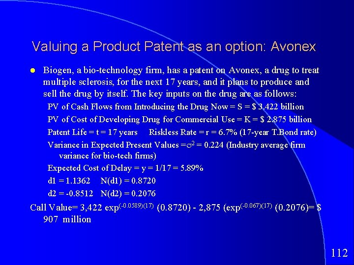
Valuing a Product Patent as an option: Avonex Biogen, a bio-technology firm, has a patent on Avonex, a drug to treat multiple sclerosis, for the next 17 years, and it plans to produce and sell the drug by itself. The key inputs on the drug are as follows: PV of Cash Flows from Introducing the Drug Now = S = $ 3. 422 billion PV of Cost of Developing Drug for Commercial Use = K = $ 2. 875 billion Patent Life = t = 17 years Riskless Rate = r = 6. 7% (17 -year T. Bond rate) Variance in Expected Present Values = 2 = 0. 224 (Industry average firm variance for bio-tech firms) Expected Cost of Delay = 1/17 = 5. 89% d 1 = 1. 1362 N(d 1) = 0. 8720 d 2 = -0. 8512 N(d 2) = 0. 2076 Call Value= 3, 422 exp(-0. 0589)(17) (0. 8720) - 2, 875 (exp(-0. 067)(17) (0. 2076)= $ 907 million 112

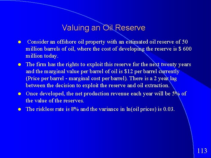
Valuing an Oil Reserve Consider an offshore oil property with an estimated oil reserve of 50 million barrels of oil, where the cost of developing the reserve is $ 600 million today. The firm has the rights to exploit this reserve for the next twenty years and the marginal value per barrel of oil is $12 per barrel currently (Price per barrel - marginal cost per barrel). There is a 2 year lag between the decision to exploit the reserve and oil extraction. Once developed, the net production revenue each year will be 5% of the value of the reserves. The riskless rate is 8% and the variance in ln(oil prices) is 0. 03. 113

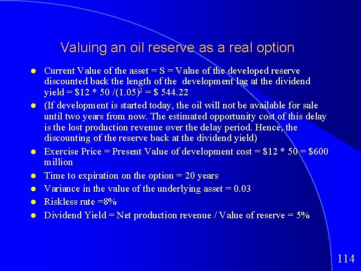
Valuing an oil reserve as a real option Current Value of the asset = S = Value of the developed reserve discounted back the length of the development lag at the dividend yield = $12 * 50 /(1. 05)2 = $ 544. 22 (If development is started today, the oil will not be available for sale until two years from now. The estimated opportunity cost of this delay is the lost production revenue over the delay period. Hence, the discounting of the reserve back at the dividend yield) Exercise Price = Present Value of development cost = $12 * 50 = $600 million Time to expiration on the option = 20 years Variance in the value of the underlying asset = 0. 03 Riskless rate =8% Dividend Yield = Net production revenue / Value of reserve = 5% 114

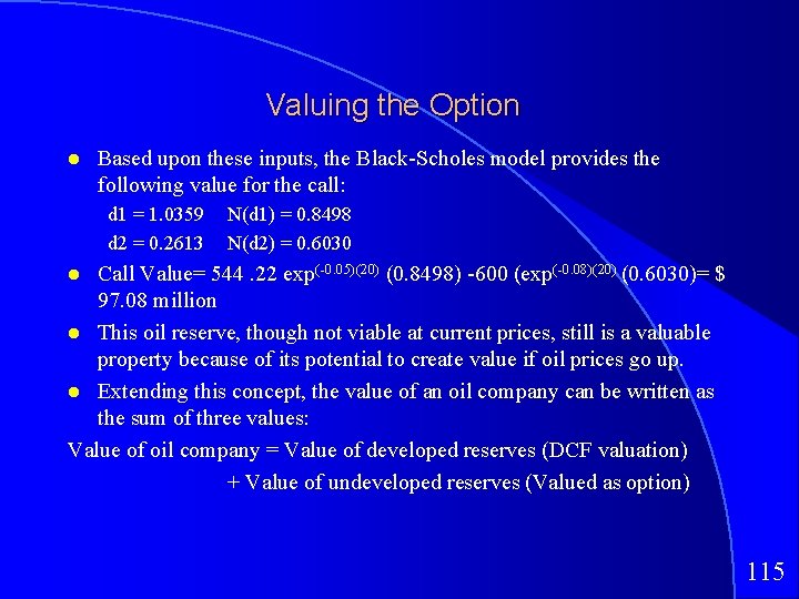
Valuing the Option Based upon these inputs, the Black-Scholes model provides the following value for the call: d 1 = 1. 0359 d 2 = 0. 2613 N(d 1) = 0. 8498 N(d 2) = 0. 6030 Call Value= 544. 22 exp(-0. 05)(20) (0. 8498) -600 (exp(-0. 08)(20) (0. 6030)= $ 97. 08 million This oil reserve, though not viable at current prices, still is a valuable property because of its potential to create value if oil prices go up. Extending this concept, the value of an oil company can be written as the sum of three values: Value of oil company = Value of developed reserves (DCF valuation) + Value of undeveloped reserves (Valued as option) 115

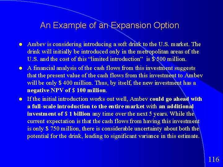
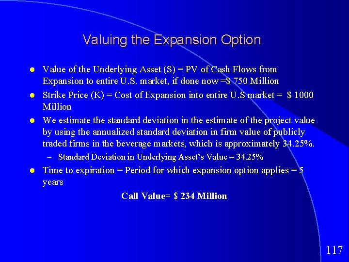
An Example of an Expansion Option Ambev is considering introducing a soft drink to the U. S. market. The drink will initially be introduced only in the metropolitan areas of the U. S. and the cost of this “limited introduction” is $ 500 million. A financial analysis of the cash flows from this investment suggests that the present value of the cash flows from this investment to Ambev will be only $ 400 million. Thus, by itself, the new investment has a negative NPV of $ 100 million. If the initial introduction works out well, Ambev could go ahead with a full-scale introduction to the entire market with an additional investment of $ 1 billion any time over the next 5 years. While the current expectation is that the cash flows from having this investment is only $ 750 million, there is considerable uncertainty about both the potential for the drink, leading to significant variance in this estimate. 116

Valuing the Expansion Option Value of the Underlying Asset (S) = PV of Cash Flows from Expansion to entire U. S. market, if done now =$ 750 Million Strike Price (K) = Cost of Expansion into entire U. S market = $ 1000 Million We estimate the standard deviation in the estimate of the project value by using the annualized standard deviation in firm value of publicly traded firms in the beverage markets, which is approximately 34. 25%. – Standard Deviation in Underlying Asset’s Value = 34. 25% Time to expiration = Period for which expansion option applies = 5 years Call Value= $ 234 Million 117

One final example: Equity as a Liquidatiion Option 118

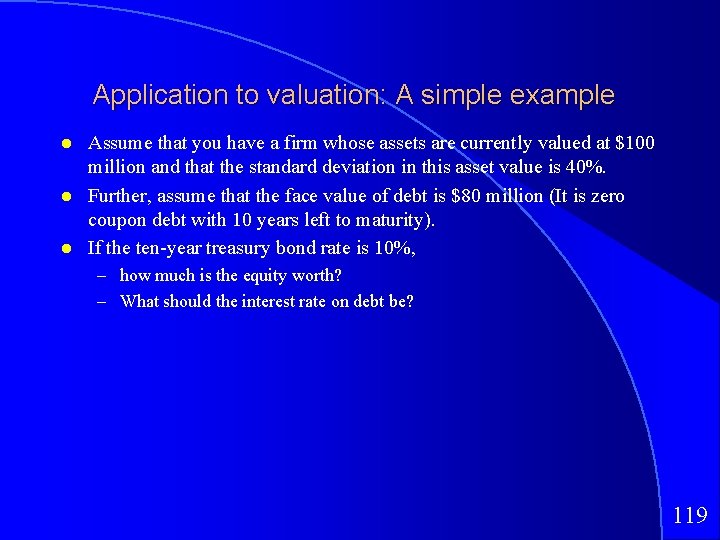
Application to valuation: A simple example Assume that you have a firm whose assets are currently valued at $100 million and that the standard deviation in this asset value is 40%. Further, assume that the face value of debt is $80 million (It is zero coupon debt with 10 years left to maturity). If the ten-year treasury bond rate is 10%, – how much is the equity worth? – What should the interest rate on debt be? 119

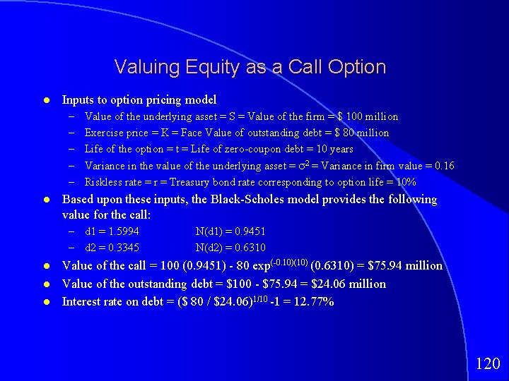
Valuing Equity as a Call Option Inputs to option pricing model – – – Value of the underlying asset = S = Value of the firm = $ 100 million Exercise price = K = Face Value of outstanding debt = $ 80 million Life of the option = t = Life of zero-coupon debt = 10 years Variance in the value of the underlying asset = 2 = Variance in firm value = 0. 16 Riskless rate = r = Treasury bond rate corresponding to option life = 10% Based upon these inputs, the Black-Scholes model provides the following value for the call: – d 1 = 1. 5994 – d 2 = 0. 3345 N(d 1) = 0. 9451 N(d 2) = 0. 6310 Value of the call = 100 (0. 9451) - 80 exp(-0. 10)(10) (0. 6310) = $75. 94 million Value of the outstanding debt = $100 - $75. 94 = $24. 06 million Interest rate on debt = ($ 80 / $24. 06)1/10 -1 = 12. 77% 120

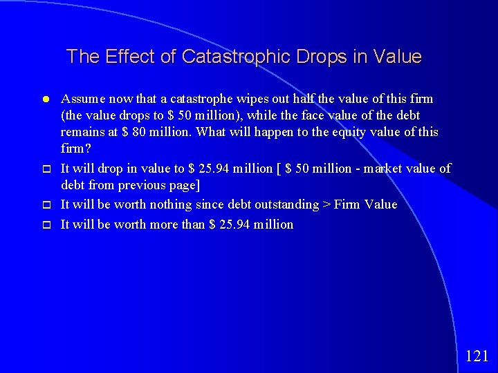
The Effect of Catastrophic Drops in Value Assume now that a catastrophe wipes out half the value of this firm (the value drops to $ 50 million), while the face value of the debt remains at $ 80 million. What will happen to the equity value of this firm? It will drop in value to $ 25. 94 million [ $ 50 million - market value of debt from previous page] It will be worth nothing since debt outstanding > Firm Value It will be worth more than $ 25. 94 million 121

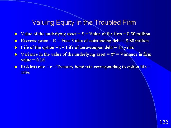
Valuing Equity in the Troubled Firm Value of the underlying asset = S = Value of the firm = $ 50 million Exercise price = K = Face Value of outstanding debt = $ 80 million Life of the option = t = Life of zero-coupon debt = 10 years Variance in the value of the underlying asset = 2 = Variance in firm value = 0. 16 Riskless rate = r = Treasury bond rate corresponding to option life = 10% 122

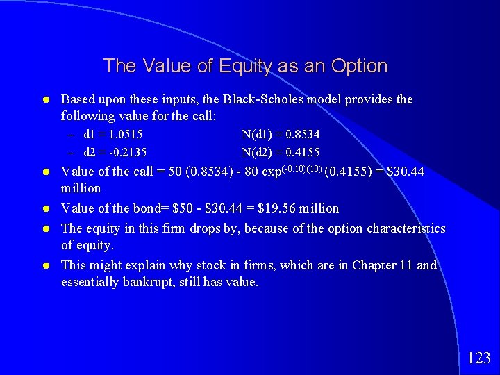
The Value of Equity as an Option Based upon these inputs, the Black-Scholes model provides the following value for the call: – d 1 = 1. 0515 – d 2 = -0. 2135 N(d 1) = 0. 8534 N(d 2) = 0. 4155 Value of the call = 50 (0. 8534) - 80 exp(-0. 10)(10) (0. 4155) = $30. 44 million Value of the bond= $50 - $30. 44 = $19. 56 million The equity in this firm drops by, because of the option characteristics of equity. This might explain why stock in firms, which are in Chapter 11 and essentially bankrupt, still has value. 123

Equity value persists. . 124

Obtaining option pricing inputs in the real worlds 125

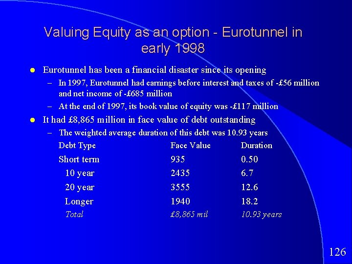
Valuing Equity as an option - Eurotunnel in early 1998 Eurotunnel has been a financial disaster since its opening – In 1997, Eurotunnel had earnings before interest and taxes of -£ 56 million and net income of -£ 685 million – At the end of 1997, its book value of equity was -£ 117 million It had £ 8, 865 million in face value of debt outstanding – The weighted average duration of this debt was 10. 93 years Debt Type Face Value Duration Short term 10 year 20 year Longer Total 935 2435 3555 1940 0. 50 6. 7 12. 6 18. 2 £ 8, 865 mil 10. 93 years 126

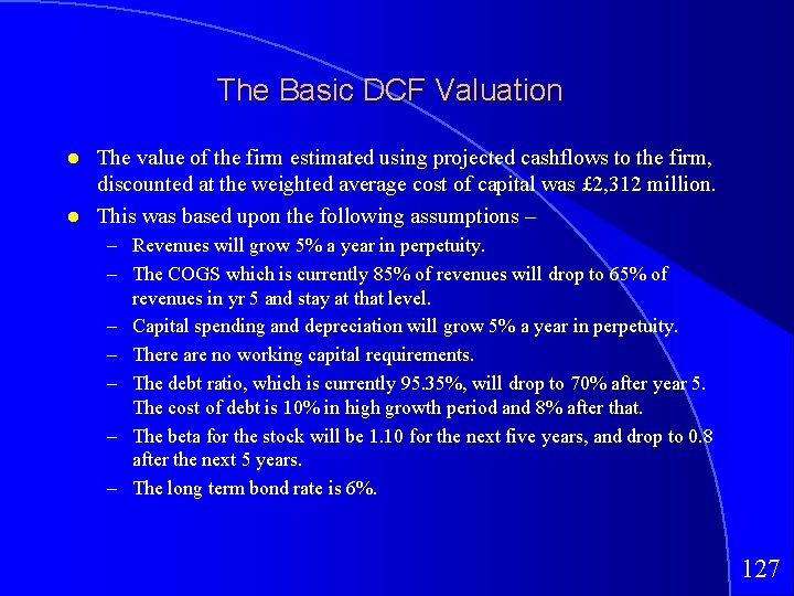
The Basic DCF Valuation The value of the firm estimated using projected cashflows to the firm, discounted at the weighted average cost of capital was £ 2, 312 million. This was based upon the following assumptions – – Revenues will grow 5% a year in perpetuity. – The COGS which is currently 85% of revenues will drop to 65% of revenues in yr 5 and stay at that level. – Capital spending and depreciation will grow 5% a year in perpetuity. – There are no working capital requirements. – The debt ratio, which is currently 95. 35%, will drop to 70% after year 5. The cost of debt is 10% in high growth period and 8% after that. – The beta for the stock will be 1. 10 for the next five years, and drop to 0. 8 after the next 5 years. – The long term bond rate is 6%. 127

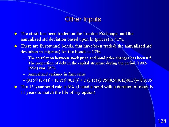
Other Inputs The stock has been traded on the London Exchange, and the annualized std deviation based upon ln (prices) is 41%. There are Eurotunnel bonds, that have been traded; the annualized std deviation in ln(price) for the bonds is 17%. – The correlation between stock price and bond price changes has been 0. 5. The proportion of debt in the capital structure during the period (19921996) was 85%. – Annualized variance in firm value = (0. 15)2 (0. 41)2 + (0. 85)2 (0. 17)2 + 2 (0. 15) (0. 85)(0. 41)(0. 17)= 0. 0335 The 15 -year bond rate is 6%. (I used a bond with a duration of roughly 11 years to match the life of my option) 128

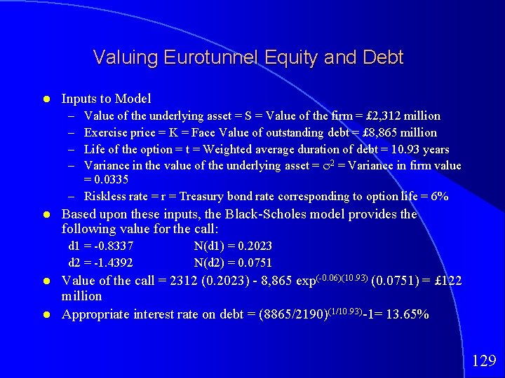
Valuing Eurotunnel Equity and Debt Inputs to Model – – Value of the underlying asset = S = Value of the firm = £ 2, 312 million Exercise price = K = Face Value of outstanding debt = £ 8, 865 million Life of the option = t = Weighted average duration of debt = 10. 93 years Variance in the value of the underlying asset = 2 = Variance in firm value = 0. 0335 – Riskless rate = r = Treasury bond rate corresponding to option life = 6% Based upon these inputs, the Black-Scholes model provides the following value for the call: d 1 = -0. 8337 d 2 = -1. 4392 N(d 1) = 0. 2023 N(d 2) = 0. 0751 Value of the call = 2312 (0. 2023) - 8, 865 exp(-0. 06)(10. 93) (0. 0751) = £ 122 million Appropriate interest rate on debt = (8865/2190)(1/10. 93)-1= 13. 65% 129

Back to Lemmings. . . 130