Valuation Techniques What is financial Value Different Views

Valuation Techniques

What is (financial) Value?

Different Views on Value “Value” refers both to general moral values and financial value. Shareholder Value in Finance assumes that shareholders are primarily interested in financial value. However, there also major shareholders who prioritize other values like - ethical investors (environment, human rights) - family owners (passing on family fortune to future generations) - governments (employment, national sovereignty) - religious institutions (religious principles) Accounting view: Value = Anchoring accounting value + Speculative value Laitoksen nimi 9. 3. 2021 3

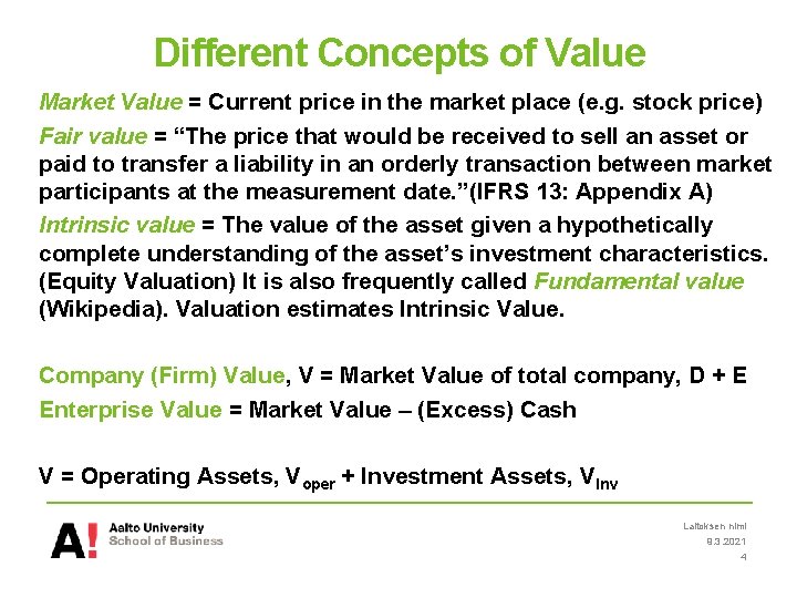
Different Concepts of Value Market Value = Current price in the market place (e. g. stock price) Fair value = “The price that would be received to sell an asset or paid to transfer a liability in an orderly transaction between market participants at the measurement date. ”(IFRS 13: Appendix A) Intrinsic value = The value of the asset given a hypothetically complete understanding of the asset’s investment characteristics. (Equity Valuation) It is also frequently called Fundamental value (Wikipedia). Valuation estimates Intrinsic Value. Company (Firm) Value, V = Market Value of total company, D + E Enterprise Value = Market Value – (Excess) Cash V = Operating Assets, Voper + Investment Assets, VInv Laitoksen nimi 9. 3. 2021 4

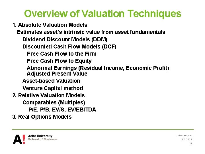
Overview of Valuation Techniques 1. Absolute Valuation Models Estimates asset’s intrinsic value from asset fundamentals Dividend Discount Models (DDM) Discounted Cash Flow Models (DCF) Free Cash Flow to the Firm Free Cash Flow to Equity Abnormal Earnings (Residual Income, Economic Profit) Adjusted Present Value Asset-based Valuation Venture Capital method 2. Relative Valuation Models Comparables (Multiples) P/E, P/B, EV/S, EV/EBITDA 3. Real Options Models Laitoksen nimi 9. 3. 2021 5

Absolute Valuation Models DDM Laitoksen nimi 9. 3. 2021 6

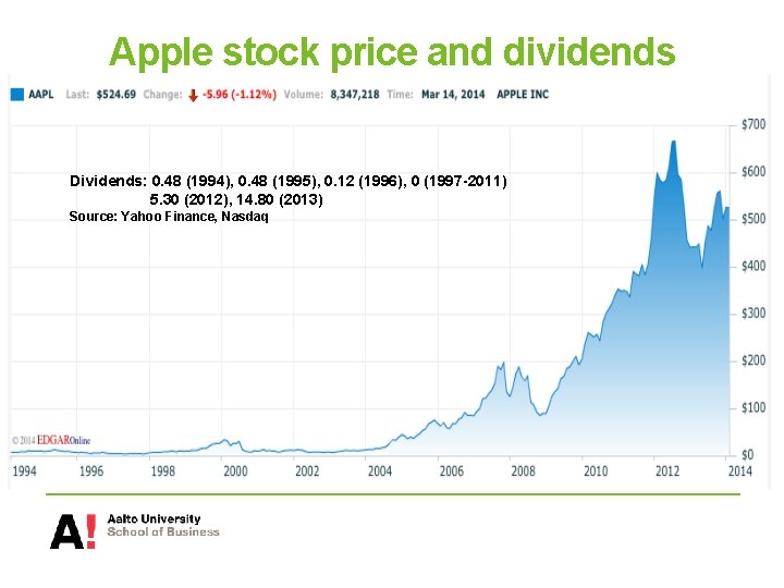
Apple stock price and dividends Dividends: 0. 48 (1994), 0. 48 (1995), 0. 12 (1996), 0 (1997 -2011) 5. 30 (2012), 14. 80 (2013) Source: Yahoo Finance, Nasdaq

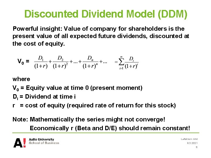
Discounted Dividend Model (DDM) Powerful insight: Value of company for shareholders is the present value of all expected future dividends, discounted at the cost of equity. V 0 = where V 0 = Equity value at time 0 (present moment) Di = Dividend at time i r = cost of equity (required rate of return for this stock) Note: Mathematically the series might not converge! Economically r (Beta and D/E) should remain constant! Laitoksen nimi 9. 3. 2021 8

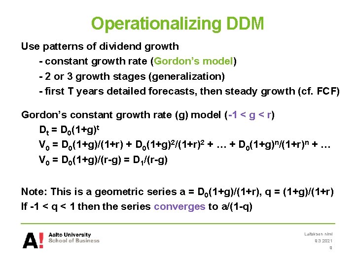
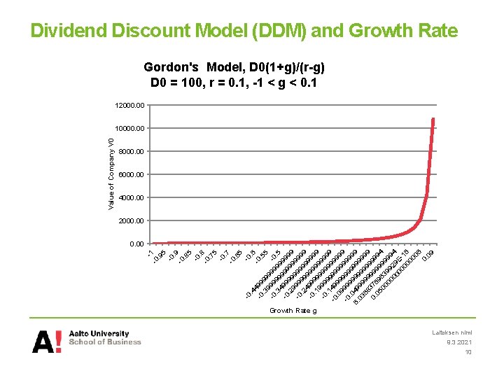
Operationalizing DDM Use patterns of dividend growth - constant growth rate (Gordon’s model) - 2 or 3 growth stages (generalization) - first T years detailed forecasts, then steady growth (cf. FCF) Gordon’s constant growth rate (g) model (-1 < g < r) Dt = D 0(1+g)t V 0 = D 0(1+g)/(1+r) + D 0(1+g)2/(1+r)2 + … + D 0(1+g)n/(1+r)n + … V 0 = D 0(1+g)/(r-g) = D 1/(r-g) Note: This is a geometric series a = D 0(1+g)/(1+r), q = (1+g)/(1+r) If -1 < q < 1 then the series converges to a/(1 -q) Laitoksen nimi 9. 3. 2021 9

-0 5 . 6. 4 4 -0 -0 99. 5. 3 99 5 99 9 -0 9 99 -0. 3 99 99. 5 4 -0 99 999. 2 99 99 9 9 -0 99 999. 2 99 99 9 4 -0 99 999. 1 99 99 9 9 -0 99 999. 1 99 99 9 -0 49 99 99. 0 99 99 9 -0 99 999. 0 99 99 9 6. 49 99 9 9 03 99 9 99 68 99 99 99 9 0. 376 999 99 05 9 9 94 00 63 99 00 99 99 00 29 4 00 E 00 16 00 06 0. 09 -0 . 7 . 6 -0 -0 5 . 8 . 7 -0 -0 5 . 9 . 8 -0 -0 5 -1. 9 -0 Value of Company V 0 Dividend Discount Model (DDM) and Growth Rate Gordon's Model, D 0(1+g)/(r-g) D 0 = 100, r = 0. 1, -1 < g < 0. 1 12000. 00 10000. 00 8000. 00 6000. 00 4000. 00 2000. 00 Growth Rate g Laitoksen nimi 9. 3. 2021 10

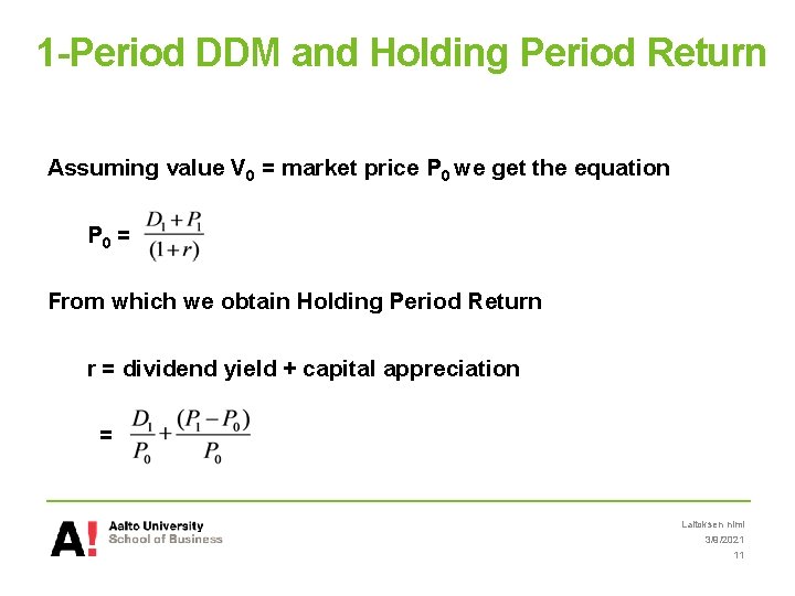
1 -Period DDM and Holding Period Return Assuming value V 0 = market price P 0 we get the equation P 0 = From which we obtain Holding Period Return r = dividend yield + capital appreciation = Laitoksen nimi 3/9/2021 11

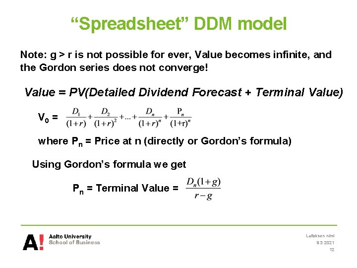
“Spreadsheet” DDM model Note: g > r is not possible for ever, Value becomes infinite, and the Gordon series does not converge! Value = PV(Detailed Dividend Forecast + Terminal Value) V 0 = where Pn = Price at n (directly or Gordon’s formula) Using Gordon’s formula we get Pn = Terminal Value = Laitoksen nimi 9. 3. 2021 12

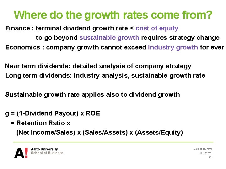
Where do the growth rates come from? Finance : terminal dividend growth rate < cost of equity to go beyond sustainable growth requires strategy change Economics : company growth cannot exceed Industry growth for ever Near term dividends: detailed analysis of company strategy Long term dividends: Industry analysis, sustainable growth rate Sustainable growth rate applies also to dividend growth g = (1 -Dividend Payout) x ROE = Retention Ratio x (Net Income/Sales) x (Sales/Assets) x (Assets/Equity) Laitoksen nimi 9. 3. 2021 13

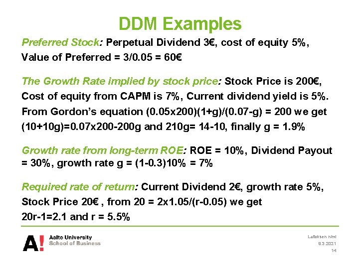
DDM Examples Preferred Stock: Perpetual Dividend 3€, cost of equity 5%, Value of Preferred = 3/0. 05 = 60€ The Growth Rate implied by stock price: Stock Price is 200€, Cost of equity from CAPM is 7%, Current dividend yield is 5%. From Gordon’s equation (0. 05 x 200)(1+g)/(0. 07 -g) = 200 we get (10+10 g)=0. 07 x 200 -200 g and 210 g= 14 -10, finally g = 1. 9% Growth rate from long-term ROE: ROE = 10%, Dividend Payout = 30%, growth rate g = (1 -0. 3)10% = 7% Required rate of return: Current Dividend 2€, growth rate 5%, Stock Price 20€ , from 20 = 2 x 1. 05/(r-0. 05) we get 20 r-1=2. 1 and r = 5. 5% Laitoksen nimi 9. 3. 2021 14

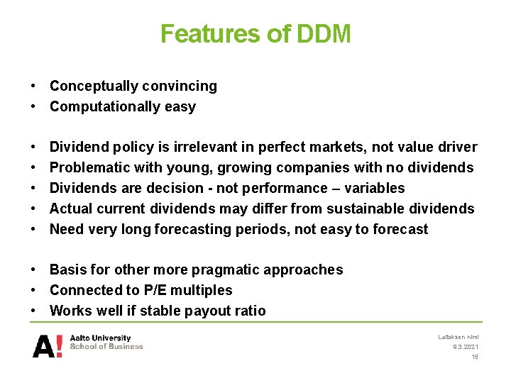
Features of DDM • Conceptually convincing • Computationally easy • • • Dividend policy is irrelevant in perfect markets, not value driver Problematic with young, growing companies with no dividends Dividends are decision - not performance – variables Actual current dividends may differ from sustainable dividends Need very long forecasting periods, not easy to forecast • Basis for other more pragmatic approaches • Connected to P/E multiples • Works well if stable payout ratio Laitoksen nimi 9. 3. 2021 15

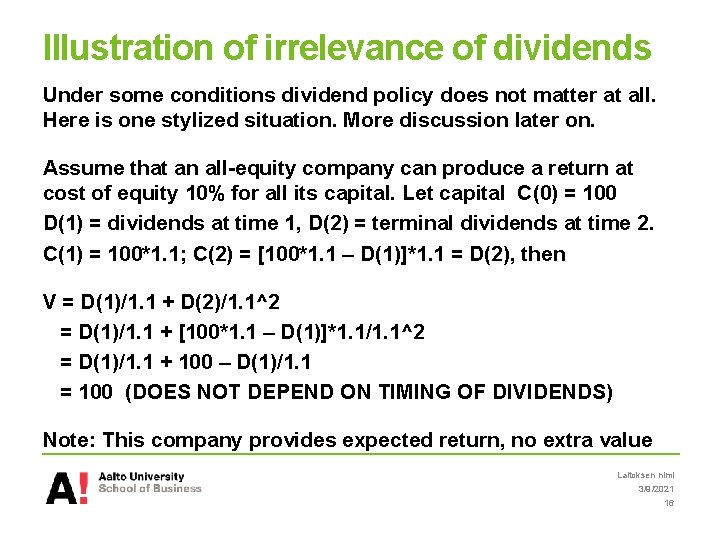
Illustration of irrelevance of dividends Under some conditions dividend policy does not matter at all. Here is one stylized situation. More discussion later on. Assume that an all-equity company can produce a return at cost of equity 10% for all its capital. Let capital C(0) = 100 D(1) = dividends at time 1, D(2) = terminal dividends at time 2. C(1) = 100*1. 1; C(2) = [100*1. 1 – D(1)]*1. 1 = D(2), then V = D(1)/1. 1 + D(2)/1. 1^2 = D(1)/1. 1 + [100*1. 1 – D(1)]*1. 1/1. 1^2 = D(1)/1. 1 + 100 – D(1)/1. 1 = 100 (DOES NOT DEPEND ON TIMING OF DIVIDENDS) Note: This company provides expected return, no extra value Laitoksen nimi 3/9/2021 16

Discounted Cash Flow Models Laitoksen nimi 9. 3. 2021 17

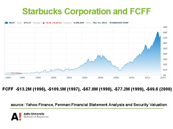
Starbucks Corporation and FCFF -$13. 2 M (1996), -$109. 5 M (1997), -$67. 0 M (1998), -$77. 2 M (1999), -$49. 6 (2000) source: Yahoo Finance, Penman: Financial Statement Analysis and Security Valuation

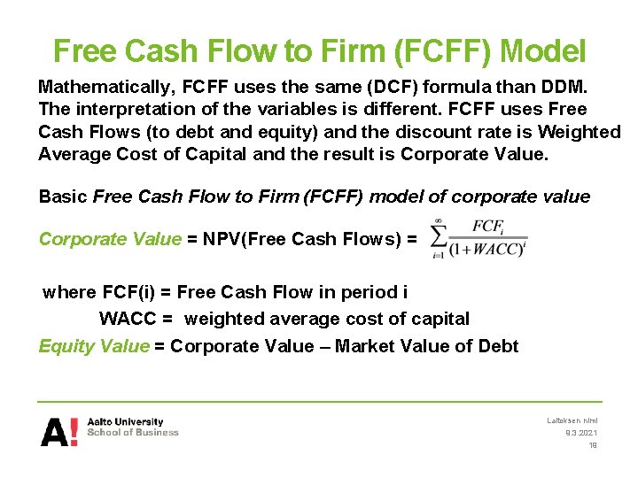
Free Cash Flow to Firm (FCFF) Model Mathematically, FCFF uses the same (DCF) formula than DDM. The interpretation of the variables is different. FCFF uses Free Cash Flows (to debt and equity) and the discount rate is Weighted Average Cost of Capital and the result is Corporate Value. Basic Free Cash Flow to Firm (FCFF) model of corporate value Corporate Value = NPV(Free Cash Flows) = where FCF(i) = Free Cash Flow in period i WACC = weighted average cost of capital Equity Value = Corporate Value – Market Value of Debt Laitoksen nimi 9. 3. 2021 19

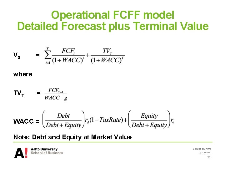
Operational FCFF model Detailed Forecast plus Terminal Value V 0 = where TVT = WACC = Note: Debt and Equity at Market Value Laitoksen nimi 9. 3. 2021 20

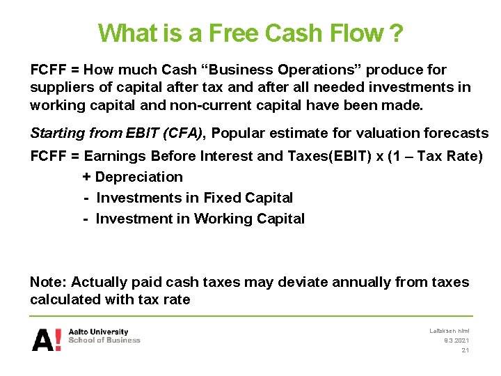
What is a Free Cash Flow ? FCFF = How much Cash “Business Operations” produce for suppliers of capital after tax and after all needed investments in working capital and non-current capital have been made. Starting from EBIT (CFA), Popular estimate for valuation forecasts FCFF = Earnings Before Interest and Taxes(EBIT) x (1 – Tax Rate) + Depreciation - Investments in Fixed Capital - Investment in Working Capital Note: Actually paid cash taxes may deviate annually from taxes calculated with tax rate Laitoksen nimi 9. 3. 2021 21

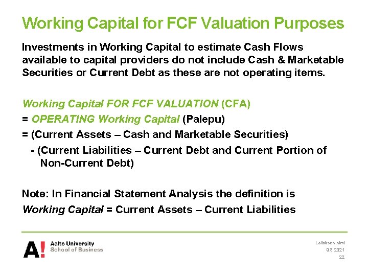
Working Capital for FCF Valuation Purposes Investments in Working Capital to estimate Cash Flows available to capital providers do not include Cash & Marketable Securities or Current Debt as these are not operating items. Working Capital FOR FCF VALUATION (CFA) = OPERATING Working Capital (Palepu) = (Current Assets – Cash and Marketable Securities) - (Current Liabilities – Current Debt and Current Portion of Non-Current Debt) Note: In Financial Statement Analysis the definition is Working Capital = Current Assets – Current Liabilities Laitoksen nimi 9. 3. 2021 22

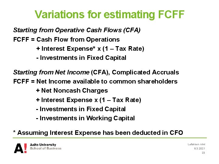
Variations for estimating FCFF Starting from Operative Cash Flows (CFA) FCFF = Cash Flow from Operations + Interest Expense* x (1 – Tax Rate) - Investments in Fixed Capital Starting from Net Income (CFA), Complicated Accruals FCFF = Net Income available to common shareholders + Net Noncash Charges + Interest Expense x (1 – Tax Rate) - Investments in Fixed Capital - Investments in Working Capital * Assuming Interest Expense has been deducted in CFO Laitoksen nimi 9. 3. 2021 23

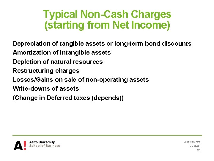
Typical Non-Cash Charges (starting from Net Income) Depreciation of tangible assets or long-term bond discounts Amortization of intangible assets Depletion of natural resources Restructuring charges Losses/Gains on sale of non-operating assets Write-downs of assets (Change in Deferred taxes (depends)) Laitoksen nimi 9. 3. 2021 24

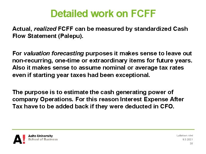
Detailed work on FCFF Actual, realized FCFF can be measured by standardized Cash Flow Statement (Palepu). For valuation forecasting purposes it makes sense to leave out non-recurring, one-time or extraordinary items for future years. Also it makes sense to assume nominal or average tax rates even if starting year taxes had been exceptional. The purpose is to estimate the cash generating power of company Operations. For this reason Interest Expense After Tax have to be added back if they were deducted in CFO. Laitoksen nimi 9. 3. 2021 25

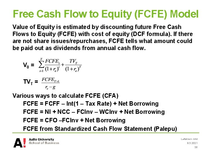
Free Cash Flow to Equity (FCFE) Model Value of Equity is estimated by discounting future Free Cash Flows to Equity (FCFE) with cost of equity (DCF formula). If there are not share issues/repurchases, FCFE tells what amount could be paid out as dividends from annual cash flow. V 0 = TVT = Various ways to calculate FCFE (CFA) FCFE = FCFF – Int(1 – Tax Rate) + Net Borrowing FCFE = NI + NCC – FCInv – WCInv + Net Borrowing FCFE = CFO –FCInv + Net Borrowing FCFE from Standardized Cash Flow Statement (Palepu) Laitoksen nimi 9. 3. 2021 26

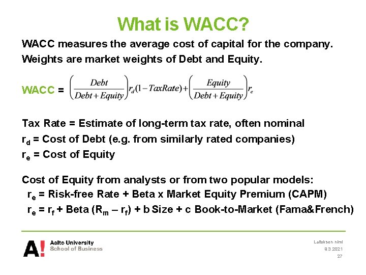
What is WACC? WACC measures the average cost of capital for the company. Weights are market weights of Debt and Equity. WACC = Tax Rate = Estimate of long-term tax rate, often nominal rd = Cost of Debt (e. g. from similarly rated companies) re = Cost of Equity from analysts or from two popular models: re = Risk-free Rate + Beta x Market Equity Premium (CAPM) re = rf + Beta (Rm – rf) + b Size + c Book-to-Market (Fama&French) Laitoksen nimi 9. 3. 2021 27

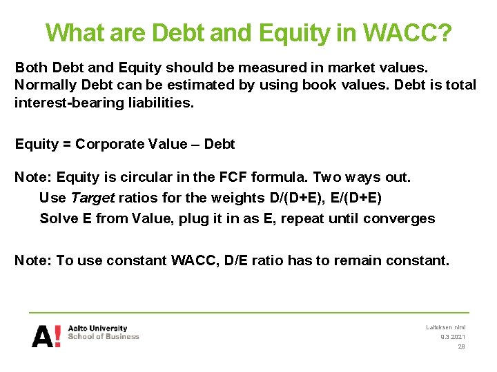
What are Debt and Equity in WACC? Both Debt and Equity should be measured in market values. Normally Debt can be estimated by using book values. Debt is total interest-bearing liabilities. Equity = Corporate Value – Debt Note: Equity is circular in the FCF formula. Two ways out. Use Target ratios for the weights D/(D+E), E/(D+E) Solve E from Value, plug it in as E, repeat until converges Note: To use constant WACC, D/E ratio has to remain constant. Laitoksen nimi 9. 3. 2021 28

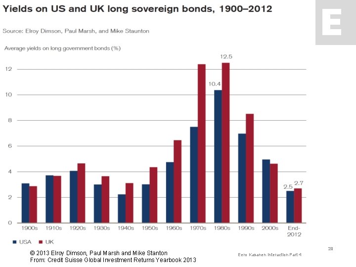
© 2013 Elroy Dimson, Paul Marsh and Mike Stanton From: Credit Suisse Global Investment Returns Yearbook 2013 29 Eero Kasanen Interaction Part 4

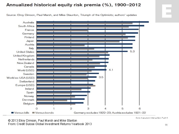
© 2013 Elroy Dimson, Paul Marsh and Mike Stanton From: Credit Suisse Global Investment Returns Yearbook 2013 Eero Kasanen Interaction Part 4 30

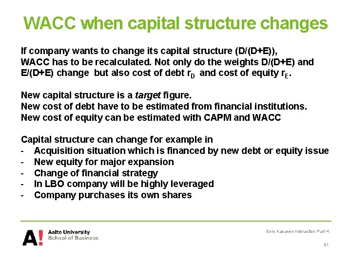
WACC when capital structure changes If company wants to change its capital structure (D/(D+E)), WACC has to be recalculated. Not only do the weights D/(D+E) and E/(D+E) change but also cost of debt r. D and cost of equity r. E. New capital structure is a target figure. New cost of debt have to be estimated from financial institutions. New cost of equity can be estimated with CAPM and WACC Capital structure can change for example in - Acquisition situation which is financed by new debt or equity issue - New equity for major expansion - Change of financial strategy - In LBO company will be highly leveraged - Company purchases its own shares Eero Kasanen Interaction Part 4 31

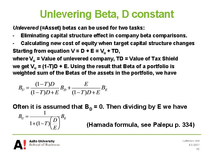
Unlevering Beta, D constant Unlevered (=Asset) betas can be used for two tasks: - Eliminating capital structure effect in company beta comparisons. - Calculating new cost of equity when target capital structure changes Starting from equation V = D + E = Vu + TD, where Vu = Value of unlevered company, TD = Value of Tax Shield we get Vu = (1 -T)D + E. Using the result that Beta of a portfolio is weighted sum of the Betas of the assets in the portfolio, we have Often it is assumed that BD = 0. Then dividing by E we have (Hamada formula, see Palepu p. 334) Laitoksen nimi 9. 3. 2021 32

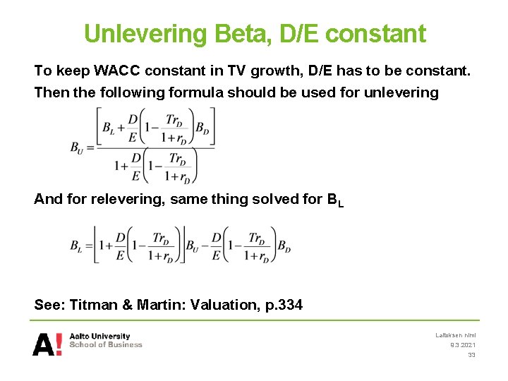
Unlevering Beta, D/E constant To keep WACC constant in TV growth, D/E has to be constant. Then the following formula should be used for unlevering And for relevering, same thing solved for BL See: Titman & Martin: Valuation, p. 334 Laitoksen nimi 9. 3. 2021 33

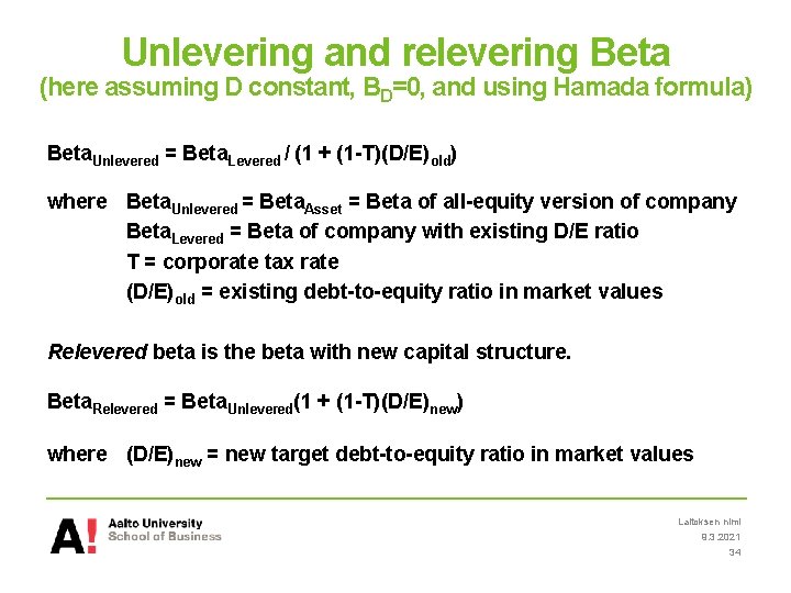
Unlevering and relevering Beta (here assuming D constant, BD=0, and using Hamada formula) Beta. Unlevered = Beta. Levered / (1 + (1 -T)(D/E)old) where Beta. Unlevered = Beta. Asset = Beta of all-equity version of company Beta. Levered = Beta of company with existing D/E ratio T = corporate tax rate (D/E)old = existing debt-to-equity ratio in market values Relevered beta is the beta with new capital structure. Beta. Relevered = Beta. Unlevered(1 + (1 -T)(D/E)new) where (D/E)new = new target debt-to-equity ratio in market values Laitoksen nimi 9. 3. 2021 34

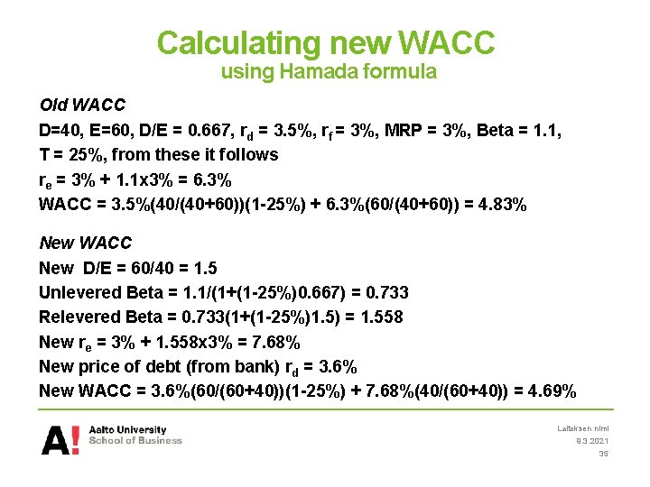
Calculating new WACC using Hamada formula Old WACC D=40, E=60, D/E = 0. 667, rd = 3. 5%, rf = 3%, MRP = 3%, Beta = 1. 1, T = 25%, from these it follows re = 3% + 1. 1 x 3% = 6. 3% WACC = 3. 5%(40/(40+60))(1 -25%) + 6. 3%(60/(40+60)) = 4. 83% New WACC New D/E = 60/40 = 1. 5 Unlevered Beta = 1. 1/(1+(1 -25%)0. 667) = 0. 733 Relevered Beta = 0. 733(1+(1 -25%)1. 5) = 1. 558 New re = 3% + 1. 558 x 3% = 7. 68% New price of debt (from bank) rd = 3. 6% New WACC = 3. 6%(60/(60+40))(1 -25%) + 7. 68%(40/(60+40)) = 4. 69% Laitoksen nimi 9. 3. 2021 35

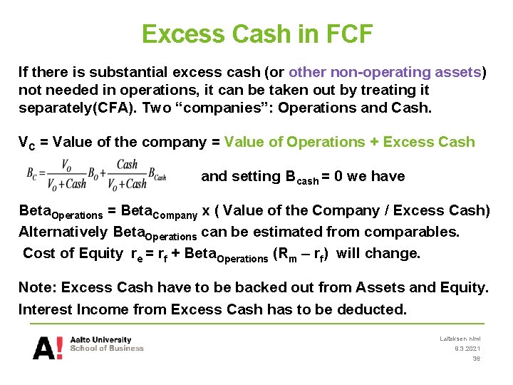
Excess Cash in FCF If there is substantial excess cash (or other non-operating assets) not needed in operations, it can be taken out by treating it separately(CFA). Two “companies”: Operations and Cash. VC = Value of the company = Value of Operations + Excess Cash and setting B cash = 0 we have Beta. Operations = Beta. Company x ( Value of the Company / Excess Cash) Alternatively Beta. Operations can be estimated from comparables. Cost of Equity re = rf + Beta. Operations (Rm – rf) will change. Note: Excess Cash have to be backed out from Assets and Equity. Interest Income from Excess Cash has to be deducted. Laitoksen nimi 9. 3. 2021 36

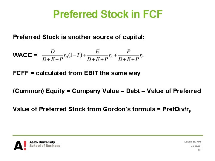
Preferred Stock in FCF Preferred Stock is another source of capital: WACC = FCFF = calculated from EBIT the same way (Common) Equity = Company Value – Debt – Value of Preferred Stock from Gordon’s formula = Pref. Div/r. P Laitoksen nimi 9. 3. 2021 37

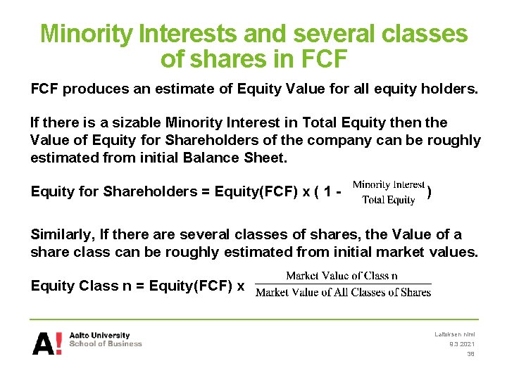
Minority Interests and several classes of shares in FCF produces an estimate of Equity Value for all equity holders. If there is a sizable Minority Interest in Total Equity then the Value of Equity for Shareholders of the company can be roughly estimated from initial Balance Sheet. Equity for Shareholders = Equity(FCF) x ( 1 - ) Similarly, If there are several classes of shares, the Value of a share class can be roughly estimated from initial market values. Equity Class n = Equity(FCF) x Laitoksen nimi 9. 3. 2021 38

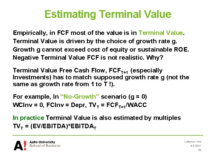
Estimating Terminal Value Empirically, in FCF most of the value is in Terminal Value is driven by the choice of growth rate g. Growth g cannot exceed cost of equity or sustainable ROE. Negative Terminal Value FCF is not realistic. Why? Terminal Value Free Cash Flow, FCFT+1 (especially Investments) has to match supposed growth rate g (not the same as growth rate from 1 to T !). For example, In “No-Growth” scenario (g = 0) WCInv = 0, FCInv = Depr, TVT = FCFT+1/WACC In practice Terminal Value is also estimated by multiples TVT = (EV/EBITDA)*EBITDAT Laitoksen nimi 9. 3. 2021 39

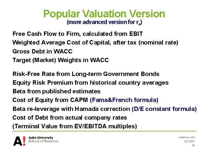
Popular Valuation Version (more advanced version for re) Free Cash Flow to Firm, calculated from EBIT Weighted Average Cost of Capital, after tax (nominal rate) Gross Debt in WACC Target (Market) Weights in WACC Risk-Free Rate from Long-term Government Bonds Equity Risk Premium from historical country averages Beta from published estimates Cost of Equity from CAPM (Fama&French formula) Beta re-leverage with Hamada correction (D/E constant formula) Cost of Debt from actual company rates (Terminal Value from EV/EBITDA multiples) Laitoksen nimi 9. 3. 2021 40

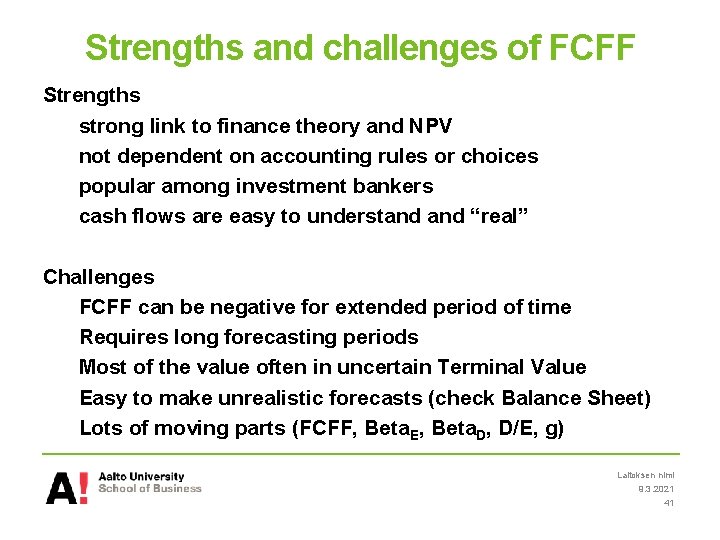
Strengths and challenges of FCFF Strengths strong link to finance theory and NPV not dependent on accounting rules or choices popular among investment bankers cash flows are easy to understand “real” Challenges FCFF can be negative for extended period of time Requires long forecasting periods Most of the value often in uncertain Terminal Value Easy to make unrealistic forecasts (check Balance Sheet) Lots of moving parts (FCFF, Beta. E, Beta. D, D/E, g) Laitoksen nimi 9. 3. 2021 41

Accruals Based Valuation Models Laitoksen nimi 9. 3. 2021 42

Discounted Abnormal Earnings Model

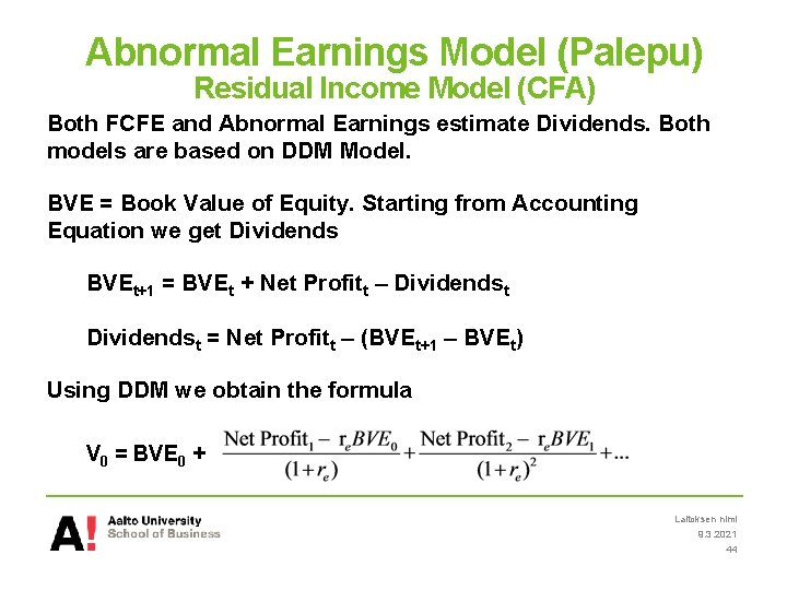
Abnormal Earnings Model (Palepu) Residual Income Model (CFA) Both FCFE and Abnormal Earnings estimate Dividends. Both models are based on DDM Model. BVE = Book Value of Equity. Starting from Accounting Equation we get Dividends BVEt+1 = BVEt + Net Profitt – Dividendst = Net Profitt – (BVEt+1 – BVEt) Using DDM we obtain the formula V 0 = BVE 0 + Laitoksen nimi 9. 3. 2021 44

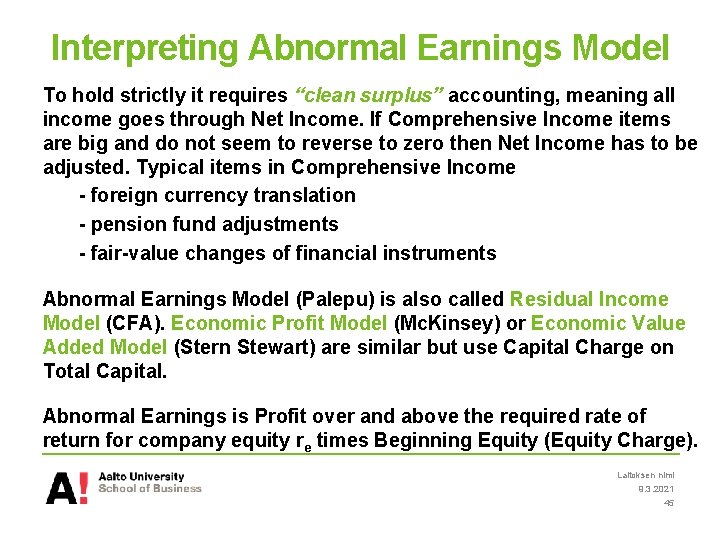
Interpreting Abnormal Earnings Model To hold strictly it requires “clean surplus” accounting, meaning all income goes through Net Income. If Comprehensive Income items are big and do not seem to reverse to zero then Net Income has to be adjusted. Typical items in Comprehensive Income - foreign currency translation - pension fund adjustments - fair-value changes of financial instruments Abnormal Earnings Model (Palepu) is also called Residual Income Model (CFA). Economic Profit Model (Mc. Kinsey) or Economic Value Added Model (Stern Stewart) are similar but use Capital Charge on Total Capital. Abnormal Earnings is Profit over and above the required rate of return for company equity re times Beginning Equity (Equity Charge). Laitoksen nimi 9. 3. 2021 45

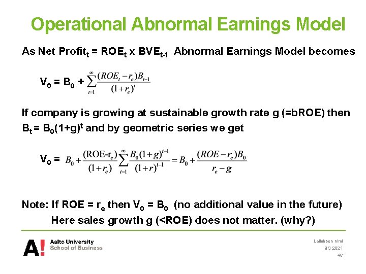
Operational Abnormal Earnings Model As Net Profitt = ROEt x BVEt-1 Abnormal Earnings Model becomes V 0 = B 0 + If company is growing at sustainable growth rate g (=b. ROE) then Bt = B 0(1+g)t and by geometric series we get V 0 = Note: If ROE = re then V 0 = B 0 (no additional value in the future) Here sales growth g (<ROE) does not matter. (why? ) Laitoksen nimi 9. 3. 2021 46

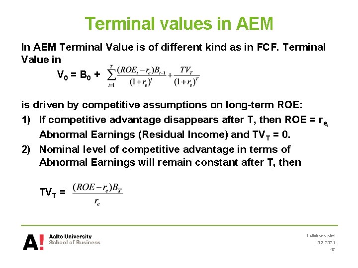
Terminal values in AEM In AEM Terminal Value is of different kind as in FCF. Terminal Value in V 0 = B 0 + is driven by competitive assumptions on long-term ROE: 1) If competitive advantage disappears after T, then ROE = re, Abnormal Earnings (Residual Income) and TVT = 0. 2) Nominal level of competitive advantage in terms of Abnormal Earnings will remain constant after T, then TVT = Laitoksen nimi 9. 3. 2021 47

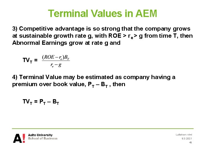
Terminal Values in AEM 3) Competitive advantage is so strong that the company grows at sustainable growth rate g, with ROE > re > g from time T, then Abnormal Earnings grow at rate g and TVT = 4) Terminal Value may be estimated as company having a premium over book value, PT – BT , then TVT = PT – BT Laitoksen nimi 9. 3. 2021 48

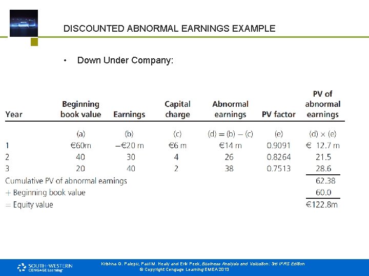
DISCOUNTED ABNORMAL EARNINGS EXAMPLE • Down Under Company: Krishna G. Palepu, Paul M. Healy and Erik Peek, Business Analysis and Valuation: 3 rd IFRS Edition © Copyright Cengage Learning EMEA 2013

Strengths and challenges of AEM(RI) Strengths: • In AEM Terminal Values are typically small • (Standardized) Accounting info can be used • Connection to competitiveness and ROE • Can be applied if DIV = 0, or FCF hard to predict or negative Challenges: • Clean Surplus condition has to hold or adjustments needed • Accounting data may need adjustments Laitoksen nimi 9. 3. 2021 50

Economic Profit Valuation Models Laitoksen nimi 9. 3. 2021 51

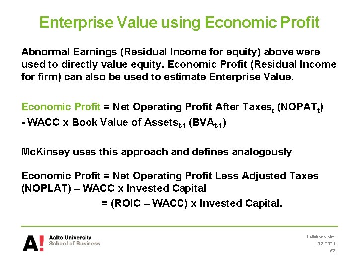
Enterprise Value using Economic Profit Abnormal Earnings (Residual Income for equity) above were used to directly value equity. Economic Profit (Residual Income for firm) can also be used to estimate Enterprise Value. Economic Profit = Net Operating Profit After Taxest (NOPATt) - WACC x Book Value of Assetst-1 (BVAt-1) Mc. Kinsey uses this approach and defines analogously Economic Profit = Net Operating Profit Less Adjusted Taxes (NOPLAT) – WACC x Invested Capital = (ROIC – WACC) x Invested Capital. Laitoksen nimi 9. 3. 2021 52

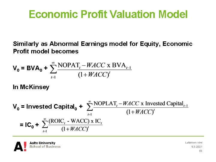
Economic Profit Valuation Model Similarly as Abnormal Earnings model for Equity, Economic Profit model becomes V 0 = BVA 0 + In Mc. Kinsey V 0 = Invested Capital 0 + = IC 0 + Laitoksen nimi 9. 3. 2021 53

Adjusted Present Value (APV) Laitoksen nimi 3/9/2021 54

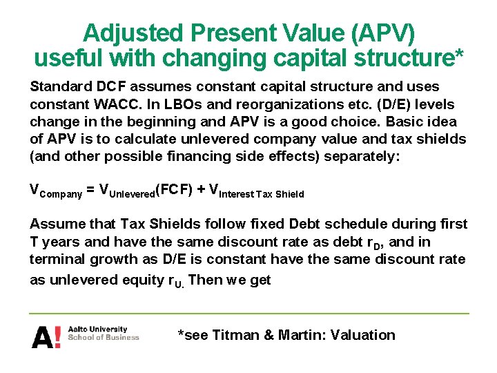
Adjusted Present Value (APV) useful with changing capital structure* Standard DCF assumes constant capital structure and uses constant WACC. In LBOs and reorganizations etc. (D/E) levels change in the beginning and APV is a good choice. Basic idea of APV is to calculate unlevered company value and tax shields (and other possible financing side effects) separately: VCompany = VUnlevered(FCF) + VInterest Tax Shield Assume that Tax Shields follow fixed Debt schedule during first T years and have the same discount rate as debt r. D, and in terminal growth as D/E is constant have the same discount rate as unlevered equity r. U. Then we get *see Titman & Martin: Valuation

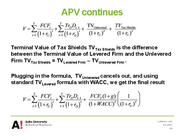
APV continues Terminal Value of Tax Shields TVTax Shields is the difference between the Terminal Value of Levered Firm and the Unlevered Firm TVTax Shields = TVLevered Firm – TVUnlevered Firm. Plugging in the formula, TVUnlevered cancels out, and using standard TVLevered formula with WACC, we get the final result Laitoksen nimi 9. 3. 2021 56

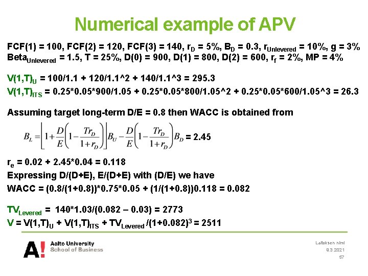
Numerical example of APV FCF(1) = 100, FCF(2) = 120, FCF(3) = 140, r. D = 5%, BD = 0. 3, r. Unlevered = 10%, g = 3% Beta. Unlevered = 1. 5, T = 25%, D(0) = 900, D(1) = 800, D(2) = 600, rf = 2%, MP = 4% V(1, T)U = 100/1. 1 + 120/1. 1^2 + 140/1. 1^3 = 295. 3 V(1, T)ITS = 0. 25*0. 05*900/1. 05 + 0. 25*0. 05*800/1. 05^2 + 0. 25*0. 05*600/1. 05^3 = 26. 3 Assuming target long-term D/E = 0. 8 then WACC is obtained from = 2. 45 re = 0. 02 + 2. 45*0. 04 = 0. 118 Expressing D/(D+E), E/(D+E) with (D/E) we have WACC = (0. 8/(1+0. 8))*0. 75*0. 05 + (1/(1+0. 8))0. 118 = 0. 082 TVLevered = 140*1. 03/(0. 082 – 0. 03) = 2773 V = V(1, T)U + V(1, T)ITS + TVLevered /(1+0. 082)3 = 2511 Laitoksen nimi 9. 3. 2021 57

Valuation using Multiples Laitoksen nimi 9. 3. 2021 58

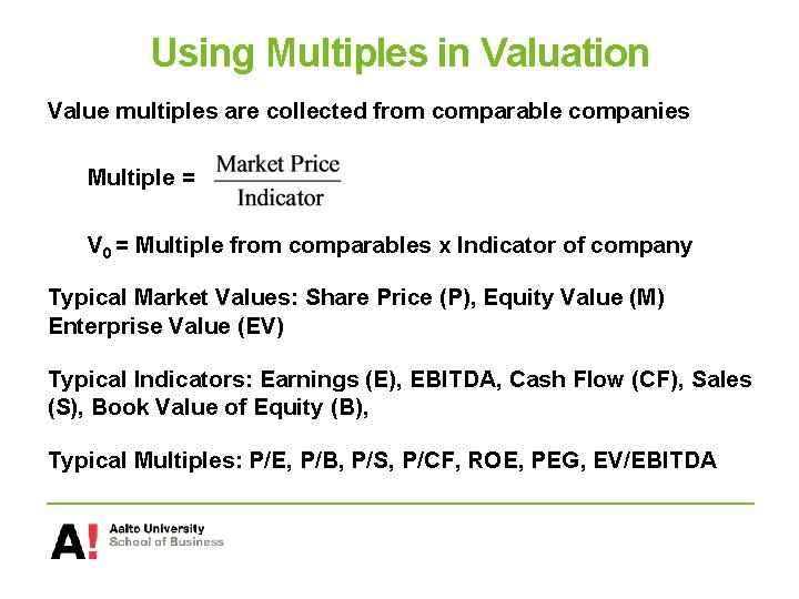
Using Multiples in Valuation Value multiples are collected from comparable companies Multiple = V 0 = Multiple from comparables x Indicator of company Typical Market Values: Share Price (P), Equity Value (M) Enterprise Value (EV) Typical Indicators: Earnings (E), EBITDA, Cash Flow (CF), Sales (S), Book Value of Equity (B), Typical Multiples: P/E, P/B, P/S, P/CF, ROE, PEG, EV/EBITDA

Operative Issues in Multiples Selection of comparables: similarity criteria – industry, country, accounting system, strategy, size, … Finding “average” of comparables : median (or weighted harmonic mean), simple average suffers from outliers Adjustments: leaving out extraordinary items, standardizing accounting practices Choices: Trailing or Forward Multiples, Basic or Diluted Earnings, Current or Smoothed Multiples DCF and AEM models provide “justified” Multiple values Laitoksen nimi 9. 3. 2021 60

Be Consistent and check definitions Several services and sources, including companies in Financial Statements, publish multiples. But P/E, M/B, EV/EBITDA differ! SAME DEFINITIONS FOR COMPANY AND ITS PEERS For example check: Gross vs Net Debt, CFO vs CF, Common vs Total Equity, Unadjusted or Adjusted Financial Statements, Undiluted or Diluted EPS, Nominal vs. Effective Tax Rates, … Stockmann 2014, Equity Ratio = (Equity plus non-controlling interests)/(Total Assets less Advance payments received) Verkkokauppa 2014, Equity Ratio = (Equity plus depreciation reserve*(1 – tax rate))/(Total sum of the balance sheet – advances received) Laitoksen nimi 9. 3. 2021 61

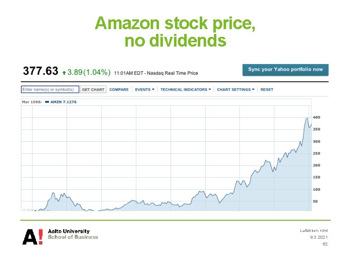
Amazon stock price, no dividends Laitoksen nimi 9. 3. 2021 62

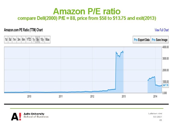
Amazon P/E ratio compare Dell(2000) P/E = 88, price from $58 to $13. 75 and exit(2013) Laitoksen nimi 9. 3. 2021 63

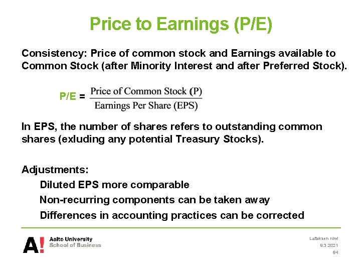
Price to Earnings (P/E) Consistency: Price of common stock and Earnings available to Common Stock (after Minority Interest and after Preferred Stock). P/E = In EPS, the number of shares refers to outstanding common shares (exluding any potential Treasury Stocks). Adjustments: Diluted EPS more comparable Non-recurring components can be taken away Differences in accounting practices can be corrected Laitoksen nimi 9. 3. 2021 64

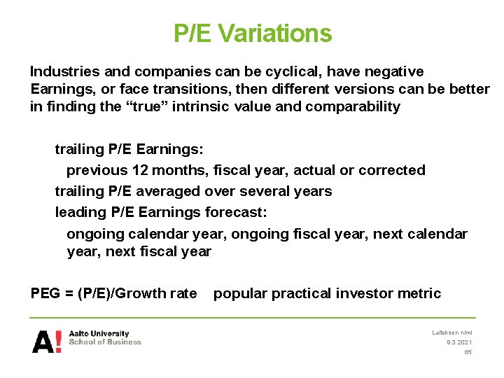
P/E Variations Industries and companies can be cyclical, have negative Earnings, or face transitions, then different versions can be better in finding the “true” intrinsic value and comparability trailing P/E Earnings: previous 12 months, fiscal year, actual or corrected trailing P/E averaged over several years leading P/E Earnings forecast: ongoing calendar year, ongoing fiscal year, next calendar year, next fiscal year PEG = (P/E)/Growth rate popular practical investor metric Laitoksen nimi 9. 3. 2021 65

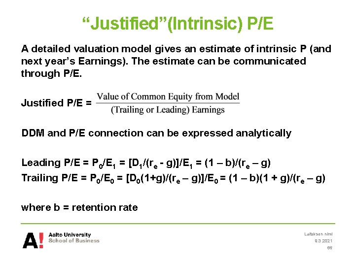
“Justified”(Intrinsic) P/E A detailed valuation model gives an estimate of intrinsic P (and next year’s Earnings). The estimate can be communicated through P/E. Justified P/E = DDM and P/E connection can be expressed analytically Leading P/E = P 0/E 1 = [D 1/(re - g)]/E 1 = (1 – b)/(re – g) Trailing P/E = P 0/E 0 = [D 0(1+g)/(re – g)]/E 0 = (1 – b)(1 + g)/(re – g) where b = retention rate Laitoksen nimi 9. 3. 2021 66

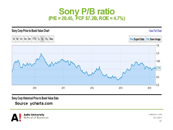
Sony P/B ratio (P/E = 20. 45, FCF $7. 2 B, ROE = 4. 7%) Source ycharts. com Laitoksen nimi 9. 3. 2021 67

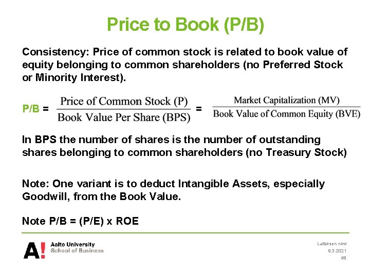
Price to Book (P/B) Consistency: Price of common stock is related to book value of equity belonging to common shareholders (no Preferred Stock or Minority Interest). P/B = = In BPS the number of shares is the number of outstanding shares belonging to common shareholders (no Treasury Stock) Note: One variant is to deduct Intangible Assets, especially Goodwill, from the Book Value. Note P/B = (P/E) x ROE Laitoksen nimi 9. 3. 2021 68

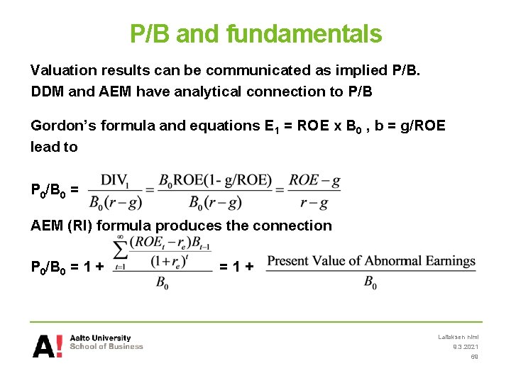
P/B and fundamentals Valuation results can be communicated as implied P/B. DDM and AEM have analytical connection to P/B Gordon’s formula and equations E 1 = ROE x B 0 , b = g/ROE lead to P 0/B 0 = AEM (RI) formula produces the connection P 0/B 0 = 1 + =1+ Laitoksen nimi 9. 3. 2021 69

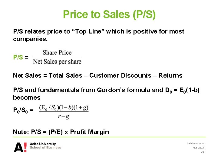
Price to Sales (P/S) P/S relates price to “Top Line” which is positive for most companies. P/S = Net Sales = Total Sales – Customer Discounts – Returns P/S and fundamentals from Gordon’s formula and D 0 = E 0(1 -b) becomes P 0/S 0 = Note: P/S = (P/E) x Profit Margin Laitoksen nimi 9. 3. 2021 70

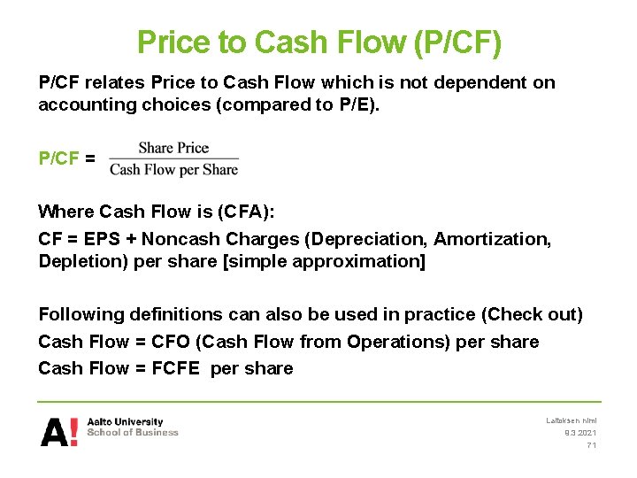
Price to Cash Flow (P/CF) P/CF relates Price to Cash Flow which is not dependent on accounting choices (compared to P/E). P/CF = Where Cash Flow is (CFA): CF = EPS + Noncash Charges (Depreciation, Amortization, Depletion) per share [simple approximation] Following definitions can also be used in practice (Check out) Cash Flow = CFO (Cash Flow from Operations) per share Cash Flow = FCFE per share Laitoksen nimi 9. 3. 2021 71

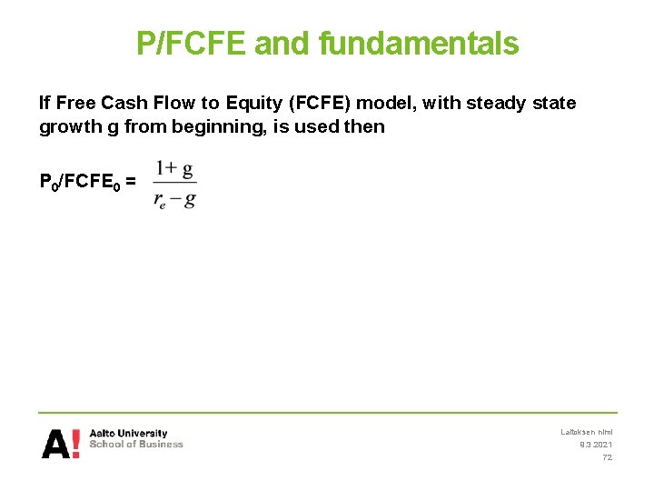
P/FCFE and fundamentals If Free Cash Flow to Equity (FCFE) model, with steady state growth g from beginning, is used then P 0/FCFE 0 = Laitoksen nimi 9. 3. 2021 72

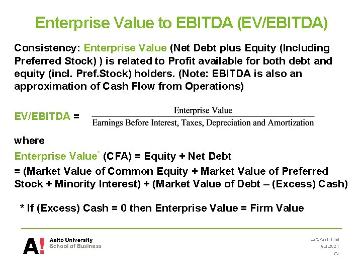
Enterprise Value to EBITDA (EV/EBITDA) Consistency: Enterprise Value (Net Debt plus Equity (Including Preferred Stock) ) is related to Profit available for both debt and equity (incl. Pref. Stock) holders. (Note: EBITDA is also an approximation of Cash Flow from Operations) EV/EBITDA = where Enterprise Value* (CFA) = Equity + Net Debt = (Market Value of Common Equity + Market Value of Preferred Stock + Minority Interest) + (Market Value of Debt – (Excess) Cash) * If (Excess) Cash = 0 then Enterprise Value = Firm Value Laitoksen nimi 9. 3. 2021 73

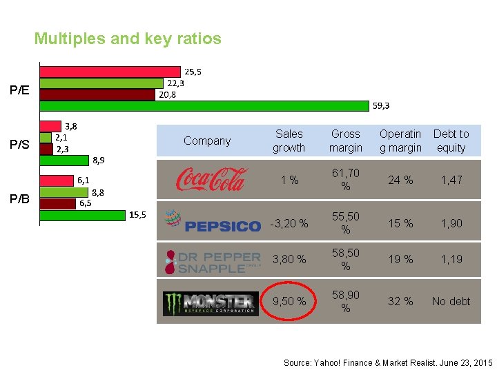
Multiples and key ratios P/E P/S Company Sales growth Gross margin Operatin g margin Debt to equity 1% 61, 70 % 24 % 1, 47 -3, 20 % 55, 50 % 15 % 1, 90 3, 80 % 58, 50 % 19 % 1, 19 9, 50 % 58, 90 % 32 % No debt P/B Source: Yahoo! Finance & Market Realist. June 23, 2015

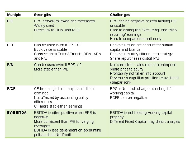
Multiple Strengths Challenges P/E EPS actively followed and forecasted Widely used Direct link to DDM and ROE EPS can be negative or zero making P/E unusable Hard to distinguish ”Recurring” and ”Nonrecurring” earnings Hard to compare internationally P/B Can be used even if EPS < 0 Book value is stable Connection to Fama&French, DDM, AEM and P/E Book values do not account for human capital and brands Book values may differ due to strategy Share repurchases distort P/B P/S Can be used even if EPS < 0 More stable than P/E Not consistent: sales refers to enterprise, share price to equity Profitability not taken into account Revenue recognition practices may distort comparisons P/CF CF less subject to manipulation than earnings Not affected by accounting policy differences CF more stable than earnings EPS + Noncash charges is not right for working capital FCFE can be negative EV/EBITDA is often positive when EPS is negative More consistent than P/E for varying leverages EBITDA is less dependent on accounting policies than Net Profit EBITDA is not treating working capital properly Different Fixed Capital may distort analysis

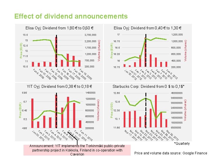
Effect of dividend announcements 2, 700, 000 17 1, 200, 000 13 2, 200, 000 16. 75 1, 000 1, 700, 000 12 1, 200, 000 11. 5 11 700, 000 10. 5 200, 000 Fe Fe Fe b b b b b 1 1 1 1 9, 20 0, 2 1, 2 2, 2 3, 2 6, 2 7, 2 8, 2 9, 2 09 00 00 9 9 9 9 5. 45 800000 600000 5. 2 400000 4. 95 Ja n 200000 Fe Fe 30 b 2, b 3, b 4, b 5, b 6, b 9, b 10 b 11 , 2 2 2 2 , , 01 015 015 015 201 5 5 5 Fe Fe 16 400, 000 Ja 200, 000 Fe Fe n n 30 31 b 1, b 2, b 3, b 6, b 7, b 8, b 9, , 2 20 20 01 01 12 12 2 2 Ja Fe Fe Fe 40000000 35000000 Price (USD) 1000000 600, 000 12. 85 Volume (shares) Price (EUR) 1200000 16. 25 Starbucks Corp: Dividend from 0 $ to 0, 1$* 1400000 5. 7 800, 000 15. 75 YIT Oyj: Dividend from 0, 38 € to 0, 18 € 5. 95 16. 5 12. 6 30000000 25000000 12. 35 20000000 15000000 12. 1 Volume (shares) 12. 5 Price (EUR) 13. 5 Volume (shares) Elisa Oyj: Dividend from 0, 40 € to 1, 30 € Volume (shares) Price (EUR) Elisa Oyj: Dividend from 1, 80 € to 0, 60 € 10000000 11. 85 M Announcement: YIT implements the Torkinmäki public-private partnership project in Kokkola, Finland in co-operation with Caverion ar 5000000 M M M ar ar 17 18 19 22 23 24 25 26 29 , 2 , 2 , 2 01 01 01 0 0 0 0 0 M ar M *Quarterly Price and volume data source: Google Finance

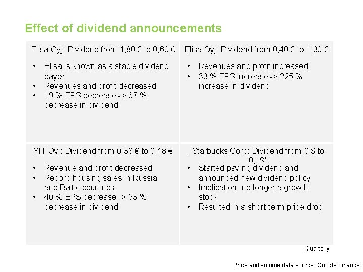
Effect of dividend announcements Elisa Oyj: Dividend from 1, 80 € to 0, 60 € • • • Elisa is known as a stable dividend payer Revenues and profit decreased 19 % EPS decrease -> 67 % decrease in dividend YIT Oyj: Dividend from 0, 38 € to 0, 18 € • • • Revenue and profit decreased Record housing sales in Russia and Baltic countries 40 % EPS decrease -> 53 % decrease in dividend Elisa Oyj: Dividend from 0, 40 € to 1, 30 € • • Revenues and profit increased 33 % EPS increase -> 225 % increase in dividend Starbucks Corp: Dividend from 0 $ to 0, 1$* • Started paying dividend announced new dividend policy • Implication: no longer a growth stock • Resulted in a short-term price drop *Quarterly Price and volume data source: Google Finance

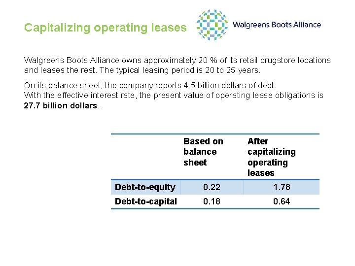
Capitalizing operating leases Walgreens Boots Alliance owns approximately 20 % of its retail drugstore locations and leases the rest. The typical leasing period is 20 to 25 years. On its balance sheet, the company reports 4. 5 billion dollars of debt. With the effective interest rate, the present value of operating lease obligations is 27. 7 billion dollars. Based on balance sheet After capitalizing operating leases Debt-to-equity 0. 22 1. 78 Debt-to-capital 0. 18 0. 64

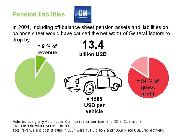
Pension liabilities In 2001, including off-balance-sheet pension assets and liabilities on balance sheet would have caused the net worth of General Motors to drop by = 9 % of revenue billion USD 13. 4 = 1565 USD per vehicle = 84 % of gross profit Note: including only Automotive, Communication services, and Other Operations. GM sold 8. 56 million vehicles in 2001. Total revenue and cost of sales in 2001 were 151. 5 billion, and 135. 6 billion USD, respectively.

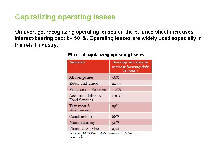
Capitalizing operating leases On average, recognizing operating leases on the balance sheet increases interest-bearing debt by 58 %. Operating leases are widely used especially in the retail industry. Effect of capitalizing operating leases

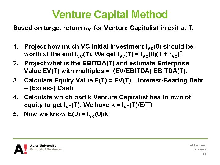
Venture Capital Method Based on target return r. VC for Venture Capitalist in exit at T. 1. Project how much VC initial investment IVC(0) should be worth at the end IVC(T). We get IVC(T) = IVC(0)(1 + r. VC)T 2. Project what is the EBITDA(T) and estimate Enterprise Value EV(T) with multiples = (EV/EBITDA) EBITDA(T). 3. Calculate Equity Value E(T) = EV(T) – Interest-Bearing Debt – (Excess) Cash 4. Calculate which part k Venture Capitalist has to own of equity to get IVC(T). We have k = IVC(T)/E(T) 5. Now we know E(0) = IVC(0)/k Laitoksen nimi 9. 3. 2021 81

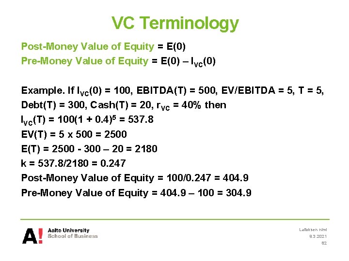
VC Terminology Post-Money Value of Equity = E(0) Pre-Money Value of Equity = E(0) – IVC(0) Example. If IVC(0) = 100, EBITDA(T) = 500, EV/EBITDA = 5, T = 5, Debt(T) = 300, Cash(T) = 20, r. VC = 40% then IVC(T) = 100(1 + 0. 4)5 = 537. 8 EV(T) = 5 x 500 = 2500 E(T) = 2500 - 300 – 20 = 2180 k = 537. 8/2180 = 0. 247 Post-Money Value of Equity = 100/0. 247 = 404. 9 Pre-Money Value of Equity = 404. 9 – 100 = 304. 9 Laitoksen nimi 9. 3. 2021 82