The Modeling of Singledof Mechanical Systems Lagrange equation

The Modeling of Single-dof Mechanical Systems

Lagrange equation for a single-dof system: (1) where: q: is the generalized coordinate; T: is the total kinetic energy of the system; V: is the total potential energy of the system; L: is the Lagrangian of the system, given by

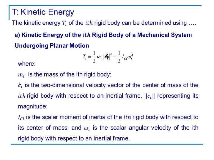
The kinetic energy of the overall system is the sum of the kinetic energies of all r rigid bodies, i. e. ,

The velocity vector of the center of mass of each body and its scalar angular velocity can be always written as linear functions of the generalized speed. The total kinetic energy of the system takes the form: (2)

V: Potential Energy In setting up the Lagrange equations of the system under study, we need an expression for its potential energy. Here, we assume that we have two possible sources of potential energy: elastic and gravitational.

Thus, under the assumption that the system has a total of s springs, the total potential energy is given as

Π and D : Power Supplied to a System and Dissipation Function

Systems are not only acted upon by driving forces but also by dissipative forces that intrinsically oppose the motion of the system. Dissipation of energy occurs in nature in many forms. The most common mechanisms of energy dissipation are: (a) viscous damping, (c) hysteretic damping, (b) Coulomb or dry-friction damping,

The Seven Steps of the Modeling Process We derive below the general form of the Lagrange equations, Eq. (1), as pertaining to single-dof systems. To this end, we use Eq. (2) to derive the Lagrangian in the form Hence, and

Likewise, In summary, then, the Lagrange equation for single-dof systems takes the form Moreover, the right-hand side of Eq. (1) is nothing but the sum of the terms due to force-controlled sources and dissipation, i. e, Therefore, the Lagrange equations take the form In summary, the Lagrange equation for single-dof systems takes the form

the governing model is a second-order ordinary differential equation in the generalized coordinate q. In this equation, the configuration-dependent coefficient m(q), the generalized mass, while the second term of the left-hand side, h(q, ˙q), contains inertia forces stemming from Coriolis and centrifugal accelerations. For this reason, this term is sometimes called the term of Coriolis and centrifugal forces. The right-hand side, in turn, is the sum of four different generalized-force terms, namely, (1) φp(q, t), a generalized force stemming from the potential energy of the Lagrangian; (2) φm(q, ˙ q, t), a generalized force stemming from motion-controlled sources and contributed by the Lagrangian as well; (3) φ f (q, ˙ q, t), a generalized force stemming from force-controlled sources, and contributed by the power Π; (4) φd (q, ˙ q, t), a generalized force of dissipative forces, stemming from the dissipation function Δ.

Example 1. 6. 4 from Dynamics Response … by J. Angeles A Locomotive Wheel Array Derive the Lagrange equation of the system shown in Fig. This system consists of two identical wheels of mass m and radius a that can be modeled as uniform disks. Furthermore, the two wheels are coupled by a slender, uniform, rigid bar of mass M and length l, pinned to the wheels at points a distance b from the wheel centers. We can safely assume that the wheels roll without slipping on the horizontal rail and that the only nonnegligible dissipative effects arise from the lubricant at the barwheel pins. These pins produce dissipative moments proportional to the relative angular velocity of the bar with respect to each wheel.

A Locomotive Wheel Array Solution: Under the no-slip assumption, it is clear that a single generalized coordinate, such as θ , suffices to describe the configuration of the entire system at any instant. The system thus has a dof = 1. We introduce the seven-step procedure to derive the mathematical model sought: 1. Kinematics 6. Power dissipation 2. Kinetic energy 7. Lagrance Equation 3. Potential energy 4. Lagrangian 5. Power supplied

A Locomotive Wheel Array 1. Kinematics. if we denote by P the center of the pin connecting the wheel 1 with the coupler bar, we have

A Locomotive Wheel Array 2. Kinetic energy

A Locomotive Wheel Array whence,

A Locomotive Wheel Array 3. Potential energy. We note that the sole source of potential energy is gravity. 4. Lagrangian. This is now readily derived as

A Locomotive Wheel Array 6. Power dissipation. What is important here is to find the angular velocity of the bar with respect to each of the wheels 7. Lagrange equation. Now, all we need is to evaluate the partial derivatives involved in Eq. 1. 22, namely,

A Locomotive Wheel Array Hence, and Furthermore, the equation sought thus being Thus, the generalized mass of the system is

A Locomotive Wheel Array Likewise, the term of Coriolis and centrifugal forces is readily identified as

Example 1. 6. 5 from Dynamics Response … by J. Angeles An Overhead Crane Now we want to derive the Lagrange equation of the overhead crane of Fig. 1. 19 that consists of a cart of mass M that is driven with a controlled motion u(t). A slender rod of length l and mass m is pinned to the cart at point O by means of roller bearings producing a resistive torque that can be assumed to be equivalent to that of a linear dashpot of coefficient c.

An Overhead Crane Solution: We proceed as in the foregoing example, in seven steps, namely, 1. Kinematics 6. Power dissipation 2. Kinetic energy 7. Lagrance Equation 3. Potential energy 4. Lagrangian 5. Power supplied 1. Kinematics

An Overhead Crane

An Overhead Crane and hence, Compared with Eq. 1. 27, the foregoing expression yields

An Overhead Crane 3. Potential energy. This is only gravitational and pertains to the rod, the potential energy of the cart remaining constant, and, therefore, can be assumed to be zero. Hence, if we use the level of the pin as a reference, 4. Lagrangian. This is simply

An Overhead Crane 6. Power dissipation. Here, the only sink of energy occurs in the pin, and hence, 7. Lagrange equations. Now it is a simplematter to calculate the partial derivatives of the foregoing functions:

An Overhead Crane Therefore, the governing equation becomes that can be rearranged in the form

An Overhead Crane Now we can readily identify the generalized mass as Likewise, and so, the system at hand contains neither Coriolis nor centrifugal forces.

An Overhead Crane

Example 1. 6. 6 from Dynamics Response … by J. Angeles A Force-driven Overhead Crane

A Force-driven Overhead Crane all other terms remaining the same. Therefore, the governing equation becomes now

Example 1. 6. 8 from Dynamics Response … by J. Angeles A Simplified Model of an Actuator Shown in Fig. is the iconic model of an actuator used to rotate a load—e. g. , a control surface in an aircraft, a robot link, a door, or a valve—of mass m, represented by link AB of length a, about a point A. The driving mechanism consists of three elements in parallel, namely, a linear spring of stiffness k, a linear dashpot of coefficient c, and a hydraulic cylinder exerting a controlled force F(t), to lower or raise the load. Under the assumption that the spring is unloaded when s = a, and that the link is a slender rod, find the mathematical model of the foregoing system in terms of θ , which is to be used as the generalized coordinate in this example.

A Simplified Model of an Actuator Solution: We proceed as in the previous cases, i. e. , following the usual seven-step procedure: 1. Kinematics 6. Power dissipation 2. Kinetic energy 7. Lagrance Equation 3. Potential energy 4. Lagrangian 5. Power supplied

A Simplified Model of an Actuator 1. Kinematics Besides the foregoing item, we will need a relation between the length of the spring, s, and the generalized variable, θ. This is readily found from the geometry of Fig. 1. 21, namely, 2. Kinetic energy.

A Simplified Model of an Actuator Thus, 3. Potential energy. We now have both gravitational and elastic forms of potential energy. If we take the horizontal position of AB as the reference level to measure the potential energy due to gravity, then

A Simplified Model of an Actuator or, in terms of the generalized coordinate alone, 4. Lagrangian. This is simply 5. Power supplied. The system is driven under a controlled force F(t) that is applied at a speed ˙ s, and hence, the power supplied to the system is

A Simplified Model of an Actuator thereby obtaining the desired expression: 6. Power dissipation. Power is dissipated only by the dashpot of the hydraulic cylinder, and hence,

A Simplified Model of an Actuator 7. Lagrange equations. We first evaluate the partial derivatives of the Lagrangian: where we have written all partial derivatives in terms of angle θ /2. Furthermore,

A Simplified Model of an Actuator the equation sought thus being The generalized mass can be readily identified from the above model as Also note that the generalized-force terms are identified below as: while

A Simplified Model of an Actuator Finally, the equation of motion can be rearranged as

Example 1. 6. 9 from Dynamics Response … by J. Angeles Motion-driven Control Surface Shown in Fig. is a highly simplified model of the actuator mechanism of an aircraft control surfacee. g. , ailerons, rudder, etc. In the model, a massless slider is positioned by a stepper motor at a displacement u(t). The inertia of the actuator-aileron system is lumped in the rigid, slender, uniform bar of length l and mass m, while all the stiffness and damping is lumped in a parallel spring-dashpot array whose left end A is pinned to a second massless slider that can slide without friction on a vertical guideway. Moreover, it is known that the spring is unloaded when u = l and θ = 0. A second motor, mounted on the first slider, exerts a torque τ (t) on the bar.

Motion-driven Control Surface (c) Obtain the mathematical model of the system and identify in it the generalized forces (1) supplied by force-controlled sources; (2) supplied by motion controlled sources; (3) stemming from potentials; and (4) produced by dissipation. 1. Kinematics 5. Power supplied 2. Kinetic energy 6. Power dissipation 3. Potential energy 7. Lagrance Equation 4. Lagrangian

Motion-driven Control Surface Solution: (a) The kinetic energy of the system is that of the overhead crane of Example 1. 6. 5, except that now the cart has negligible mass, i. e. , M = 0, and hence, Moreover, from the geometry of Fig. 1. 22,

Motion-driven Control Surface whence, and

Motion-driven Control Surface (c) mathematical model of the system

Motion-driven Control Surface

Motion-driven Control Surface Thus, the mathematical model is derived as or,

Equilibrium States of Mechanical Systems we derive the equilibrium equation in the form

Example 1. 9. 1 from Dynamics Response … by J. Angeles Equilibrium Analysis of the Overhead Cran

Equilibrium Analysis of the Overhead Crane which can be written as

Equilibrium Analysis of the Overhead Crane and hence, The system, therefore, admits two equilibrium configurations, one with the rod above and one with the rod below the pin.

Equilibrium Analysis of the Overhead Crane Moreover, from Fig. 1. 30, it is apparent that

Example 1. 9. 2 from Dynamics Response … by J. Angeles Equilibrium States of the Actuator Mechanis Determine all the equilibrium states of the actuator mechanism introduced in Example 1. 6. 8. To this end, assume that

Equilibrium States of the Actuator Mechanism

Equilibrium States of the Actuator Mechanism which vanishes under any of the conditions given below:

The foregoing values yield the equilibrium configurations of Fig. 1. 31.

Example 1. 9. 4 (A System with a Time-varying Equilibrium State). Derive the equilibrium states of the rack-and-pinion transmission of Fig. 1. 3.

Moreover, no changes in the potential energy are apparent, since the center of mass of the pinion remains at the same level, and hence, we can set V = 0, which leads to L = T in this case. Now the Lagrange equation of the system is, simply,

Linearization About Equilibrium States. Stability If a system is in an equilibrium state and is perturbed slightly, then, the system may respond in one of three possible ways: • The system returns eventually to its equilibrium state • The system never returns to its equilibrium state, from which it wanders farther and farther • The system neither returns to its equilibrium state nor escapes from it; rather, the system oscillates about the equilibrium state In the first case, the equilibrium state is said to be stable or, more precisely, asymptotically stable; in the second case, the equilibrium state is unstable or asymptotically unstable. The third case is a borderline case between the two foregoing cases. This case, then, leads to what is known as a marginally stable equilibrium state.

We analyze below a single-dof system governed by the equation First, we perturb slightly the equilibrium state, Otherwise, one can resort to a series expansion.

where the subscripted vertical bar indicates that the quantity to its left is evaluated at equilibrium. At the equilibrium

Therefore, substituting Under the small-perturbation assumption, the quadratic term involving the product ………. in the left-hand side of the above equation is too small with respect to the linear terms, and hence, is neglected.

The perturbed equation of motion thus reduces to with the definitions below:

Given the linearized equation of a one-dof system, where m. E > 0, the system

For brevity , we shall write in a simpler form, i. e. , by dropping the subscript E and the δ symbol, whenever the equilibrium configuration is either self-understood or immaterial, namely, or, in normal form, as n with ωn and ζ defined now as n and, obviously, f (t) defined as

n The mathematical model appearing in Eq. 1. 57 corresponds to the iconic model of Fig. 1. 34.

A Mass-spring-dashpot System in a Gravity Field

Example 1. 10. 4 (A Mass-spring-dashpot System in a Gravity Field). Illustrated in Fig. 1. 36 is a massspring-dashpot system suspended from a rigid ceiling. For this system, discuss the difference in the models resulting when the displacement of the mass is measured (a) from the configuration where the spring is unloaded and (b) from the static equilibrium configuration. In Fig. 1. 36 a the system is displayed with the spring unloaded, while the same system is shown in its static equilibrium position in Fig. 1. 36 b, this position being that at which the spring force balances the weight of the mass, and hence, Application of Newton’s equation in the vertical direction now gives Thus, the equilibrium equation derived above reduces to

If, rather than measuring the displacement of the mass from equilibrium, we measure it from the position in which the spring is unloaded, then we set up the governing equation in terms of the new variable ξ , defined as Upon substituting in the governing equation derived above, we have

Example 1. 10. 1 from Dynamics Response … by J. Angeles Stability Analysis of the Overhead Crane Determine the stability of the equilibrium configurations of the overhead crane introduced in Example 1. 6. 5.

Stability Analysis of the Overhead Crane which leads to

Stability Analysis of the Overhead Crane Finally,

Example 1. 10. 2 from Dynamics Response … by J. Angeles Stability Analysis of the Actuator Mechanism Decide whether each of the equilibrium configurations of Fig. 1. 31, of the actuator mechanism, found in Example 1. 9. 2 is stable or unstable, when the system is unactuated—i. e. , when F(t) = 0. For the stable cases, whether stability is asymptotic or marginal, and find, in each case, the equivalent natural frequency and, if applicable, the damping ratio.

Stability Analysis of the Actuator Mechanism Solution: What we have to do is linearize the governing equation about each equilibrium configuration, with F(t) = 0. To do this, we substitute the values below into the Lagrange equation of the system at hand: The equation of motion thus becomes We analyze below each of the three equilibrium configurations found in Example 1. 9. 2:

Stability Analysis of the Actuator Mechanism the linearized equation about the equilibrium configuration considered here thus becoming, after simplifications,

Stability Analysis of the Actuator Mechanism Upon dropping the quadratic terms of the above expression, and rearranging the expression thus resulting in normal form, we obtain The natural frequency and the damping ratio associated with the linearized system are thus

Stability Analysis of the Actuator Mechanism Upon substitution of the foregoing values into the Lagrange equation, we obtain, after simplification, Next, we delete the quadratic terms from the above equation, and rewrite it in normal form, thus obtaining