Modeling of Digital Communication Systems using Simulink Chap


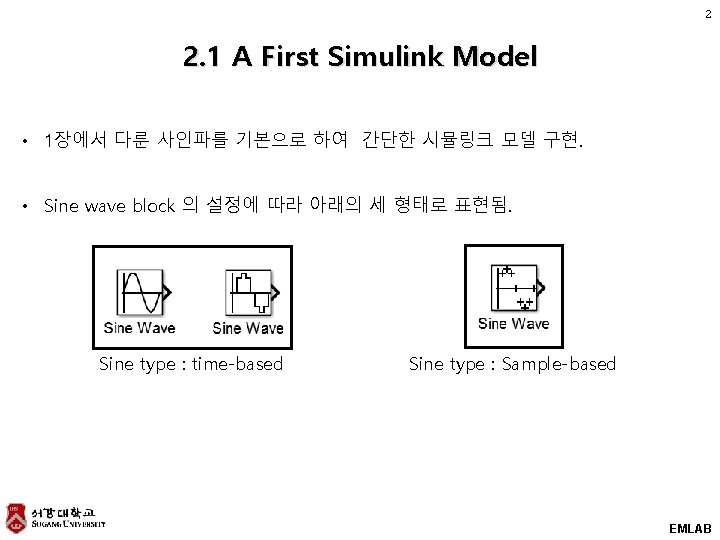
 Sine type : time based •")
 Sine type : Sample-based EMLAB")

 • Save format 을 timeseries")
 • Command 창에서 To workspace")
 • Sample time 을 0.")


 • ① • 전력 스펙트럼 [d.")
![13 2. 3 Spectrum of Sine Wave (cont’d) • ② • 스펙트럼 [d. B]](https://slidetodoc.com/presentation_image_h/2e7739caca0801eafa609996b5710baf/image-14.jpg "13 2. 3 Spectrum of Sine Wave (cont’d) • ② • 스펙트럼 [d. B]")
 • 스펙트럼 관찰 Sine wave –")

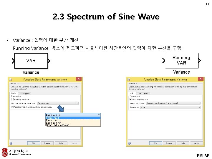
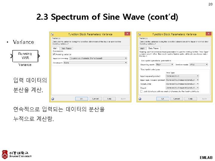
 • Variance 입력 데이터의 분산을 계산.")
 • Variance Example EMLAB")
 • Running Variance Example EMLAB")
 • Step")
 • Random")
![25 • BPSK Constellation (phase offset [rad] : 0, pi/60, pi/5 (시계방향)) EMLAB](https://slidetodoc.com/presentation_image_h/2e7739caca0801eafa609996b5710baf/image-26.jpg "25 • BPSK Constellation (phase offset [rad] : 0, pi/60, pi/5 (시계방향)) EMLAB")
 • BPSK")
 • Step")
 • Step")
 • Eb/N")
 • Step")
 Im(Output of BPSK Modulator) •")
 • Step")
 • 시뮬레이션")
 • Step")


- Slides: 44
Modeling of Digital Communication Systems using Simulink Chap 2. Sinusoidal Simulink Model Chap 3. Digital Communications BER Performance in AWGN (BPSK and QPSK) EMLAB
1 목차 Chap 2. Sinusoidal Simulink Model 2. 1 A First Simulink Model 2. 2 Simulink Model of Sine Wave 2. 3 Spectrum of a Sine Wave Chap 3. Digital Communications BER Performance in AWGN (BPSK and QPSK) 3. 1 BPSK and QPSK Error Rate Performance in AWGN 3. 2 Construction of a Simulink Model in Simple Steps 3. 3 Comparison of Simulated and Theoretical BER 3. 4 Alternate Simulink Model for BPSK 3. 5 Frame-Based Simulink Model 3. 6 QPSK Symbol Error Rate Performance 3. 7 BPSK Fixed Point Performance EMLAB
3 2. 1 A First Simulink Model (cont’d) Sine type : time based • Sine-type 이 time based 인 경우 연속 신호 및 이산 신호로 구분됨. (Sample time = 0 : continuous signal) (Sample time > 0 : discrete signal) EMLAB
4 2. 1 A First Simulink Model (cont’d) Sine type : Sample-based EMLAB
5 2. 2 Simulink Model of Sine Wave EMLAB
6 2. 2 Simulink Model of Sine Wave (cont’d) • Save format 을 timeseries 로 하면 시간정보와 함께 데이터가 저장되며 matlab command window 에서 마우스 오른쪽 > plot 메뉴가 생성됨. • Save format option: structure with time, structure, array, time series EMLAB
7 2. 2 Simulink Model of Sine Wave (cont’d) • Command 창에서 To workspace 블록 출력 (timeseries 선택 시) EMLAB
8 2. 2 Simulink Model of Sine Wave (cont’d) • Sample time 을 0. 05 → 0. 01 로 변경 • Phase shift 0 → π/2 로 변경 EMLAB
9 2. 3 Spectrum of Sine Wave EMLAB
10 2. 3 Spectrum of Sine Wave ① ② EMLAB
12 2. 3 Spectrum of Sine Wave (cont’d) • ① • 전력 스펙트럼 [d. BW] EMLAB
13 2. 3 Spectrum of Sine Wave (cont’d) • ② • 스펙트럼 [d. B] EMLAB
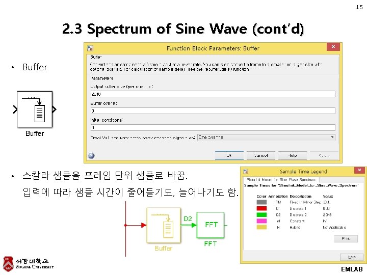
14 2. 3 Spectrum of Sine Wave (cont’d) • 스펙트럼 관찰 Sine wave – Buffer – FFT – Abs – Product – Vector scope EMLAB
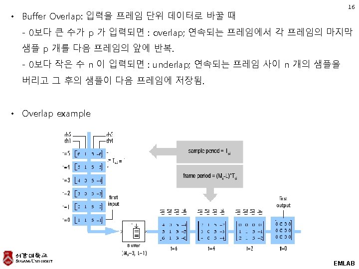
buffer overlap factor 0 17 buffer overlap factor -500 buffer overlap factor 500 EMLAB
18 2. 3 Spectrum of Sine Wave (cont’d) • Variance 입력 데이터의 분산을 계산. EMLAB
19 2. 3 Spectrum of Sine Wave (cont’d) • Variance Example EMLAB
21 2. 3 Spectrum of Sine Wave (cont’d) • Running Variance Example EMLAB
23 3. 2 Construction of a Simulink Model in Simple Steps (cont’d) • Step 1. EMLAB
24 3. 2 Construction of a Simulink Model in Simple Steps (cont’d) • Random Integer Generator Initial seed 는 임의의 소수로 선택, 이 블록의 출력은 1초에 하나씩 생성되는 0 혹은 1의 값을 갖는 샘플. • BPSK Modulator Baseband EMLAB
25 • BPSK Constellation (phase offset [rad] : 0, pi/60, pi/5 (시계방향)) EMLAB
26 3. 2 Construction of a Simulink Model in Simple Steps (cont’d) • BPSK Demodulator Baseband • Output EMLAB
27 3. 2 Construction of a Simulink Model in Simple Steps (cont’d) • Step 1 출력: 입력 데이터와 출력 데이터가 동일함. EMLAB
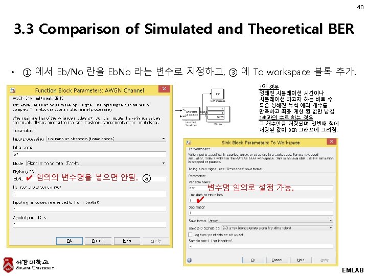
28 3. 2 Construction of a Simulink Model in Simple Steps (cont’d) • Step 2 – AWGN 블록 추가 signal routing 블록 (Goto 및 From) 을 통해 변조 전의 파형을 스코프로 관찰. • 아래와 같은 모드 선택 가능. 예제에서는 symbol period 과 sample time 이 동일하므로 Eb/N 0 = Es/N 0. EMLAB
29 3. 2 Construction of a Simulink Model in Simple Steps (cont’d) • Eb/N 0 = 100 d. B Input to BPSK Modulator Output of BPSK Demodulator Eb/N 0 = 100 d. B • Eb/N 0 = -10 d. B Input to BPSK Modulator Output of BPSK Demodulator Eb/N 0 = -10 d. B EMLAB
30 3. 2 Construction of a Simulink Model in Simple Steps (cont’d) • Step 3 – AWGN 블록 통과 전 후의 BPSK 신호 관찰. (실수/허수부) EMLAB
31 • BPSK 변조된 파형 Re(Output of BPSK Modulator) Im(Output of BPSK Modulator) • + AWGN (Eb/N 0 = 4 d. B) • BPSK 복조된 파형 Input to BPSK Modulator Output of BPSK Demodulator Eb/N 0 = 4 d. B EMLAB
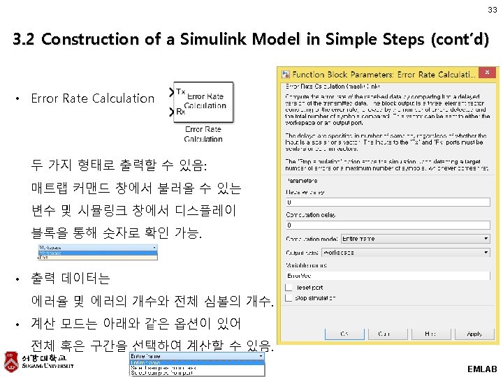
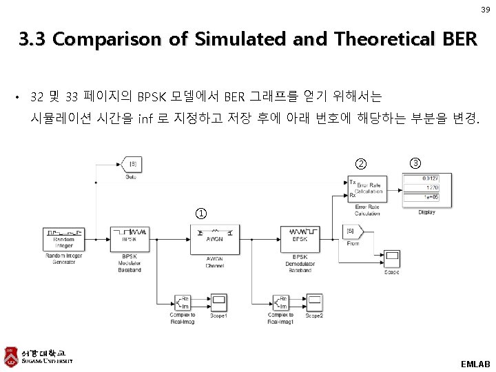
32 3. 2 Construction of a Simulink Model in Simple Steps (cont’d) • Step 4 – 에러율 계산 블록 추가 EMLAB
34 3. 2 Construction of a Simulink Model in Simple Steps (cont’d) • 시뮬레이션 시간: 100, 000 초. 초당 심볼 수 1개. • Display: BER = 0. 0127, 에러 개수 = 1270, 전체 심볼 수 = 100, 000 개. EMLAB
35 3. 2 Construction of a Simulink Model in Simple Steps (cont’d) • Step 5 – 신호와 포트의 데이터 타입 디스플레이 및 정보 블록 추가. • 시뮬링크 창의 Display>Signals&Ports>Port Data Types 선택. EMLAB
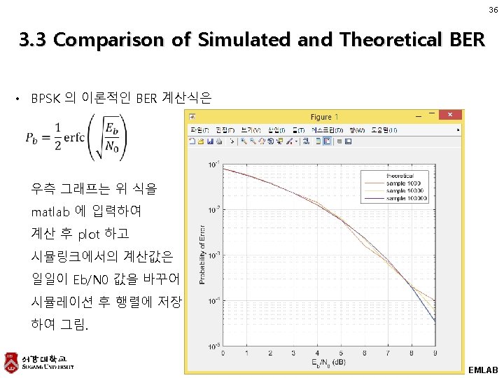
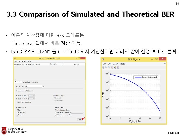
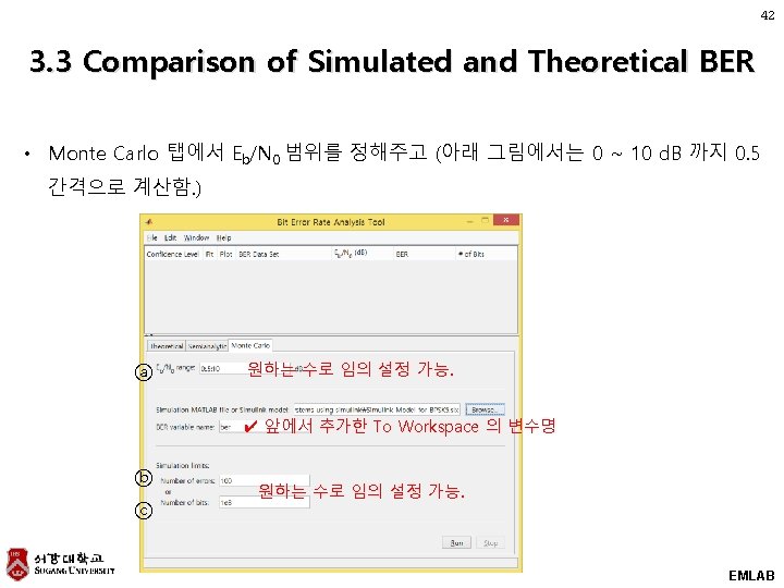
37 3. 3 Comparison of Simulated and Theoretical BER • Matlab bertool 사용법 • Matlab command 창에 bertool 입력 EMLAB
41 3. 3 Comparison of Simulated and Theoretical BER • ② 의 속성 창에서 Target number of errors 와 Maximum number of symbols 를 각각 max. Num. Errs 및 max. Num. Bits 라는 변수로 저장. ⓑ ✔ 임의의 변수명을 넣으면 안됨. ⓒ ✔ 임의의 변수명을 넣으면 안됨. EMLAB
43 3. 3 Comparison of Simulated and Theoretical BER EMLAB