Chapter 3 Mathematical Modeling of Mechanical Systems and

Chapter 3 Mathematical Modeling of Mechanical Systems and Electrical Systems

3 -1 Introduction This chapter presents mathematical modeling of mechanical systems and electrical systems. The mathematical law governing mechanical systems is Newton’s second law, while the basic laws governing the electrical circuits are Kirchhoff’s laws.

3 -2 Mathematical modeling of mechanical systems Typical mechanical systems may involve two kinds of motion: linear motion and rotational motion. Spring, mass, damper and inverted pendulum are widely used devices to describe a large class of mechanical systems. Example (Automobile suspension system). As the car moves along the road, the vertical displacements at the tires act as the motion excitation to the automobile suspension system. The motion of this system consists of

a translational motion of the center of mass and a rotational motion about the center of mass, and can be simplified as a system with springs, mass and dampers shown below.

3 -2 Mathematical modeling of mechanical systems Example. Equivalent spring constants. x k 1 F k 2 y x F k 1 k 2 Systems consisting of two springs in parallel and series, respectively.

Example. Systems consisting of two dampers connected in parallel and series, respectively. Find their equivalent viscous-friction coefficients beq with respect to dy/dt and dx/dt. (Fig. a) Solution: (a) The force f that causes the displacements is

(b): (Fig. b) The same force f is transmitted through the shaft and therefore, from which we have

Since we want to determine the relationship between dy/dt and dx/dt, that is, where beq is the equivalent viscous friction coefficient, by substituting (2) into (1) yields. Hence,

Example. Consider the spring-mass-dashpot system mounted on a massless cart. Let u, the displacement of the cart, be the input, and y, the displacement of the mass, be the output. Obtain the mathematical model of the SMD system. u y Forces acting on the mass:

By Newton’s law: Therefore, the system transfer function can be obtained as

Example. Mechanical system is shown below. Obtain the transfer functions X 1(s)/U(s) and X 2(s)/U(s), where u denotes the force, and x 1 and x 2 denote the displacements of the two carts, respectively. Solution: By Newton’s second law, we have

Simplifying, we obtain

Taking the Laplace transforms of these two equations, and assuming zero initial conditions, Solving Equation (2) for X 2(s) and substituting it into Equation (1) and simplifying, we get

Example. An inverted pendulum mounted on a motordrive cart is shown below. This is a model of attitude control of a space booster on takeoff; that is, the objective of the attitude control problem is to keep the space booster in a vertical position. u sin

Define: u: the control force to the cart; : the angle of the rod from the vertical line; (x. G, y. G): the center of gravity of the rod in (x, y) coordinates. Hence, 1) The horizontal motion of cart is described by

2)The horizontal motion of center of gravity of the rod is 3)The vertical motion of center of gravity of the pendulum rod is

4) The rotation motion of the rod about its center of gravity can be described by where I is the moment of inertia of the rod about its center of gravity. 5) Linearization of the equations (2)-(4):

Since we must keep the inverted pendulum vertical, we can assume that and d /dt are small quantities so that sin , cos 1 and (d /dt)2 0. Hence, the equations (2)-(4) can be linearized as By replacing (1) into (2) yields From equations (2)-(4), we have

From (6), we have Substituting (7) into (5) yields Taking the Laplace transform on both sides of (8) yields Therefore,

Example. An inverted pendulum is shown in the figure below. Similar to the previous example: u sin P

For this case, the moment of inertia of the pendulum about its center of gravity is small, and we assume I = 0. Then the mathematical model for this system becomes:

Example. Gear Train: Rotational transformer. In servo control systems, the rotor drives a load through gear train. N 1 Jm m m N 2 JL L, L Gear ratio (transmission ratio): where N 1 and N 2 denote the number of teeth of the two gears, respectively.

3 -3 Mathematical modeling of electrical systems 1. RLC circuit Example. RLC circuit u By using Kirchihoff’s law, we have Since we have RLC y

Example. RLC circuit. Find V(s)/R(s). r(t) Current source v(t) Taking the Laplace transform of the above equation yields

Hence,

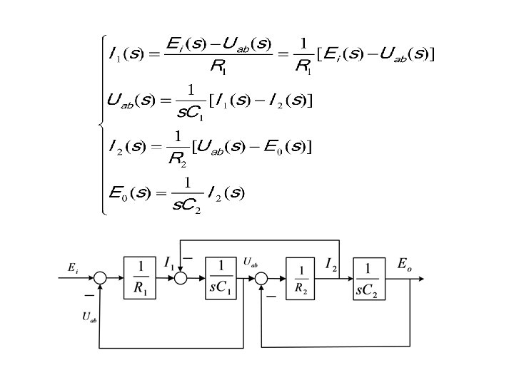
2. Transfer functions of cascaded elements Example. Find Eo(s)/Ei(s). Note that in this circuit, the second portion (R 2 C 2) produces a loading effect on the first stage (R 1 C 1 portion); that is , we cannot obtain the transfer function as we did for transfer functions in cascade.

and Taking the Laplace transforms of the above equations, we obtain

from which we obtain

The above analysis shows that, if two RC circuits connected in cascade so that the output from the first circuit is the input to the second, the overall transfer function is not the product of 1/(R 1 C 1 s+1) and 1/(R 2 C 2 s+1) due to the loading effect (a certain amount of power is withdrawn).

3. Complex impedances Resistance R: R Capacitance: 1/Cs Inductance: Ls Example. Find Y(s)/U(s) Solution:

Example. Find Eo(s)/Ei(s). Solution: Utilizing complex impedance approach, we have (from left to right)

Example. Find Eo(s)/Ei(s). C

4. Transfer functions of nonloading cascaded elements Again, consider the two simple RC circuits. Now, the circuits are isolated by an amplifier as shown below and therefore, have negligible loading effects, and the transfer function

In general, the transfer function of a system consisting of two or more nonloading cascaded elements can be obtained by eliminating the intermediate inputs and outputs: R(s) G 1(s) U G 1(s)G 2(s) C(s)

5. Operational amplifiers In the ideal op amp, no current flows into the input terminals, and the output voltage is not affected by the load connected to the output terminal. In other words, the input impedance is infinity and the output impedance is zero.

6. Examples: DC motor and servo system Example. Find the transfer function of a DC motor. Assume that the rotor has inertia Jm and viscous friction coefficient fm. Determine m(s)/Ua(s), where m is the rotational angle and ua is the power supply voltage. Ua(s) DC motor m(s)

Stator winding: 定子绕 组； Rotor windings: 转子绕 组； Shaft: 电机轴； Inertia load: 惯性负载; Bearings: 轴承 ua Commutator：换向器 m

Rotor: 转子；Torque: 电磁转矩；Back emf voltage: 反 电势； Armature current: 电枢电流; ua m m: rotational angle; ua: power supply voltage

The motor equations: 1) The electromagnetic torque Mm on the rotor in terms of the armature current ia (Cm: torque constant): 2) The back emf voltage Eb in terms of the shaft’s rotational velocity d m/dt is (Kb : electrical constant): 3) The electrical equation:

4) The torque equation: by using Newton’s law, Taking the Laplace transform of (3) and in view of (2) yields Hence, Taking the Laplace transform of (4) and in view of (1) yields

From (5) and (6), we have In particular, if La 0, we can simplify the model as where

Example. A servo system is shown below, where r and c are the input and output (that are propor-tional to the angular positions of potentiometers), e=r c, (er ec)=K 0(r c) K 0: proportionality constant; K 1: amplifier gain; eb: back emf voltage; n: gear ratio.

where in this example, for the DC motor 1) The electromagnetic torque (K 2: torque constant): 2) The back emf voltage (K 3 : electrical constant): where is the rotational angle;

3) The electrical equation: 4) The torque equation: where J 0 and b 0 denote the moment of inertia and friction constant, respectively. Then, by neglecting La, the open-loop transfer function can be simplified as

where

Summary of Chapter 3 In this chapter, we studied the mathematical modeling of some simple mechanical and electrical systems. 1. For mechanical systems, Newton’s second law is applied to establish the mathematical models of (1) some spring-mass-damper systems and (2), inverted pendulum systems.

2. For electrical systems, Kirchhoff’s laws are used. In particular, the concept of complex impedance is introduced, which provides a convenient way to obtain system transfer function.

3. The mathematical modeling of DC motor, which combines mechanical and electrical systems, is introduced and can be expressed as Ua(s) DC motor m(s)