Structural Equation Modeling Structural Equation Modeling Diagramming P

Structural Equation Modeling

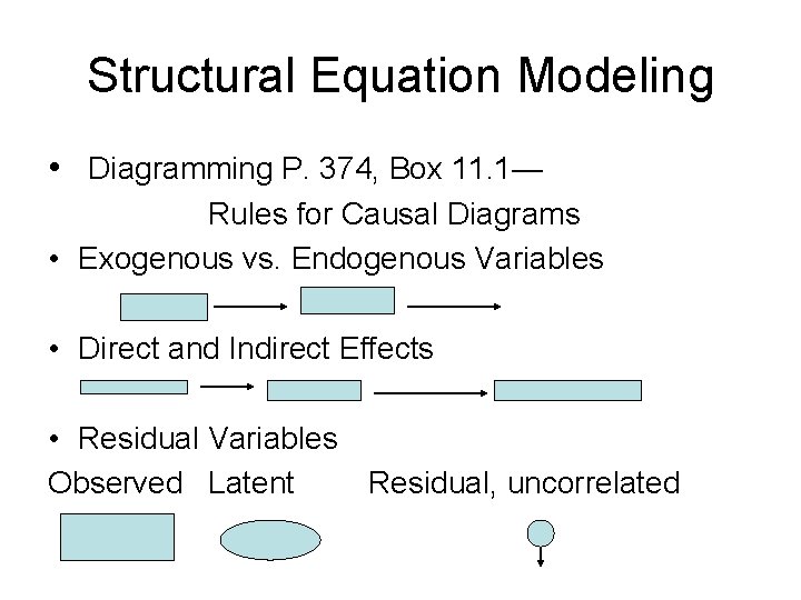
Structural Equation Modeling • Diagramming P. 374, Box 11. 1— Rules for Causal Diagrams • Exogenous vs. Endogenous Variables • Direct and Indirect Effects • Residual Variables Observed Latent Residual, uncorrelated

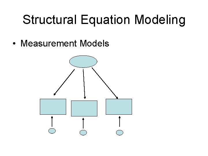
Structural Equation Modeling • Measurement Models

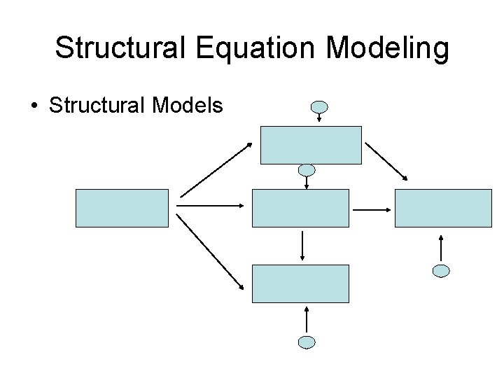
Structural Equation Modeling • Structural Models

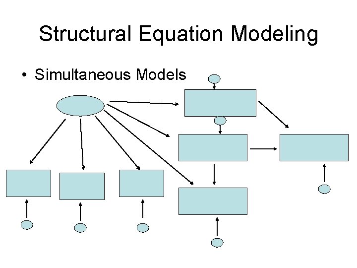
Structural Equation Modeling • Simultaneous Models

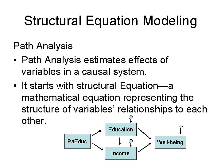
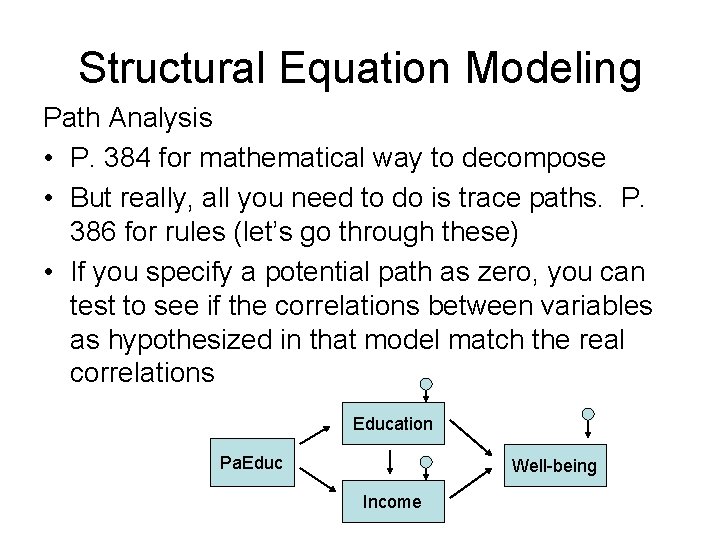
Structural Equation Modeling Path Analysis • Path Analysis estimates effects of variables in a causal system. • It starts with structural Equation—a mathematical equation representing the structure of variables’ relationships to each other. Education Pa. Educ Well-being Income

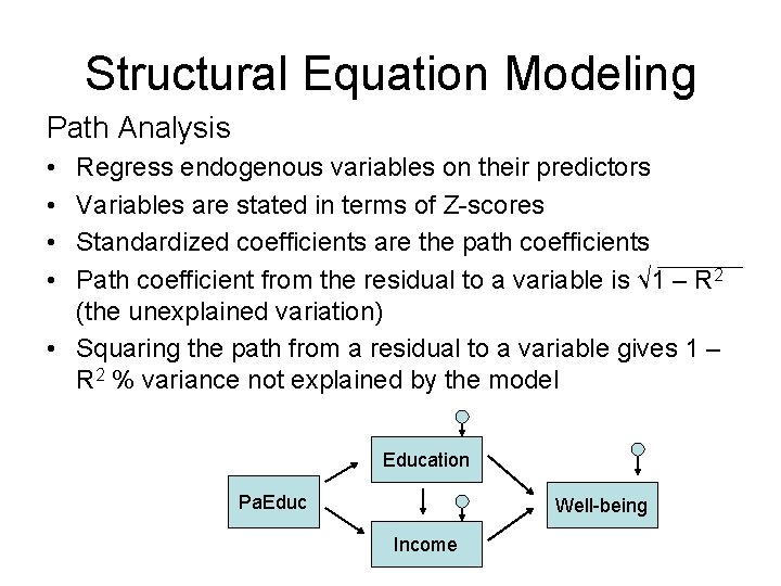
Structural Equation Modeling Path Analysis • • Regress endogenous variables on their predictors Variables are stated in terms of Z-scores Standardized coefficients are the path coefficients Path coefficient from the residual to a variable is √ 1 – R 2 (the unexplained variation) • Squaring the path from a residual to a variable gives 1 – R 2 % variance not explained by the model Education Pa. Educ Well-being Income

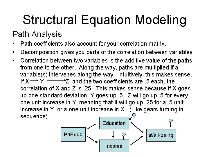
Structural Equation Modeling Path Analysis • Path coefficients also account for your correlation matrix. • Decomposition gives you parts of the correlation between variables • Correlation between two variables is the additive value of the paths from one to the other. Along the way, paths are multiplied if a variable(s) intervenes along the way. Intuitively, this makes sense. If X Y Z, and the two coefficients are. 5 each, the correlation of X and Z is. 25. This makes sense because if X goes up one standard deviation, Y goes up. 5. Z will go up. 5 for every one unit increase in Y, meaning that it will go up. 25 for a. 5 unit increase in Y, or a one unit increase in X. (Like gears turning in sequence). Education Pa. Educ Well-being Income

Structural Equation Modeling Path Analysis • P. 384 for mathematical way to decompose • But really, all you need to do is trace paths. P. 386 for rules (let’s go through these) • If you specify a potential path as zero, you can test to see if the correlations between variables as hypothesized in that model match the real correlations Education Pa. Educ Well-being Income

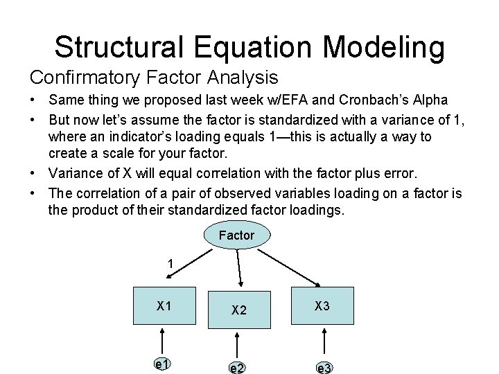
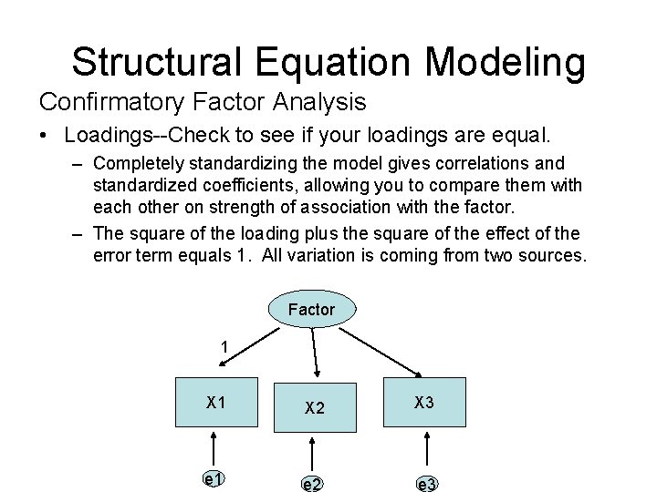
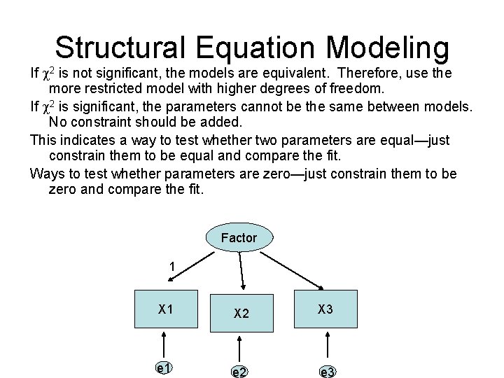
Structural Equation Modeling Confirmatory Factor Analysis • Same thing we proposed last week w/EFA and Cronbach’s Alpha • But now let’s assume the factor is standardized with a variance of 1, where an indicator’s loading equals 1—this is actually a way to create a scale for your factor. • Variance of X will equal correlation with the factor plus error. • The correlation of a pair of observed variables loading on a factor is the product of their standardized factor loadings. Factor 1 X 2 X 3 e 1 e 2 e 3

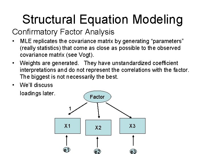
Structural Equation Modeling Confirmatory Factor Analysis • MLE replicates the covariance matrix by generating “parameters” (really statistics) that come as close as possible to the observed covariance matrix (see Vogt). • Weights are generated. They have unstandardized coefficient interpretations and do not represent the correlations with the factor. The biggest is not necessarily the best. • We’ll discuss loadings later. Factor 1 X 2 X 3 e 1 e 2 e 3

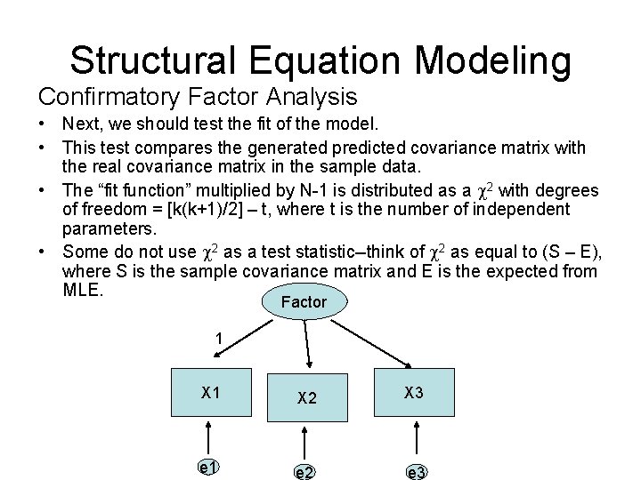
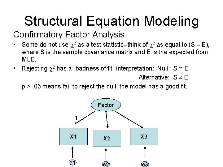
Structural Equation Modeling Confirmatory Factor Analysis • Next, we should test the fit of the model. • This test compares the generated predicted covariance matrix with the real covariance matrix in the sample data. • The “fit function” multiplied by N-1 is distributed as a 2 with degrees of freedom = [k(k+1)/2] – t, where t is the number of independent parameters. • Some do not use 2 as a test statistic--think of 2 as equal to (S – E), where S is the sample covariance matrix and E is the expected from MLE. Factor 1 X 2 X 3 e 1 e 2 e 3

Structural Equation Modeling Confirmatory Factor Analysis • Some do not use 2 as a test statistic--think of 2 as equal to (S – E), where S is the sample covariance matrix and E is the expected from MLE. • Rejecting 2 has a “badness of fit” interpretation: Null: S = E Alternative: S E p >. 05 means fail to reject the null, the model has a good fit. Factor 1 X 2 X 3 e 1 e 2 e 3

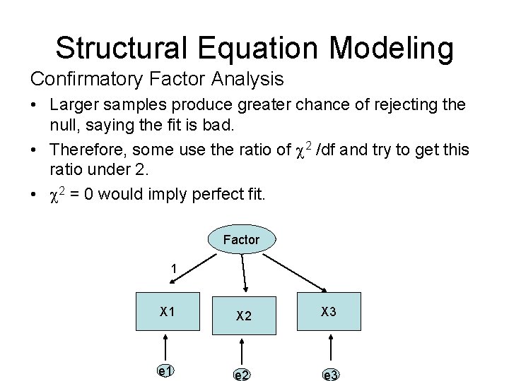
Structural Equation Modeling Confirmatory Factor Analysis • Larger samples produce greater chance of rejecting the null, saying the fit is bad. • Therefore, some use the ratio of 2 /df and try to get this ratio under 2. • 2 = 0 would imply perfect fit. Factor 1 X 2 X 3 e 1 e 2 e 3

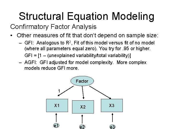
Structural Equation Modeling Confirmatory Factor Analysis • Other measures of fit that don’t depend on sample size: – GFI: Analogous to R 2, Fit of this model versus fit of no model (where all parameters equal zero). You try for. 95 or higher. GFI = [1 – (unexplained variability/total variability)] – AGFI: GFI adjusted for model complexity. More complex models reduce GFI more. Factor 1 X 2 X 3 e 1 e 2 e 3

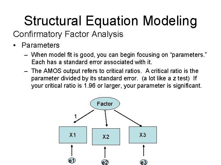
Structural Equation Modeling Confirmatory Factor Analysis • Parameters – When model fit is good, you can begin focusing on “parameters. ” Each has a standard error associated with it. – The AMOS output refers to critical ratios. A critical ratio is the parameter divided by its standard error. (a lot like a z test) If your critical ratio is 1. 96 or larger, your parameter is significant. Factor 1 X 2 X 3 e 1 e 2 e 3

Structural Equation Modeling Confirmatory Factor Analysis • Loadings--Check to see if your loadings are equal. – Completely standardizing the model gives correlations and standardized coefficients, allowing you to compare them with each other on strength of association with the factor. – The square of the loading plus the square of the effect of the error term equals 1. All variation is coming from two sources. Factor 1 X 2 X 3 e 1 e 2 e 3

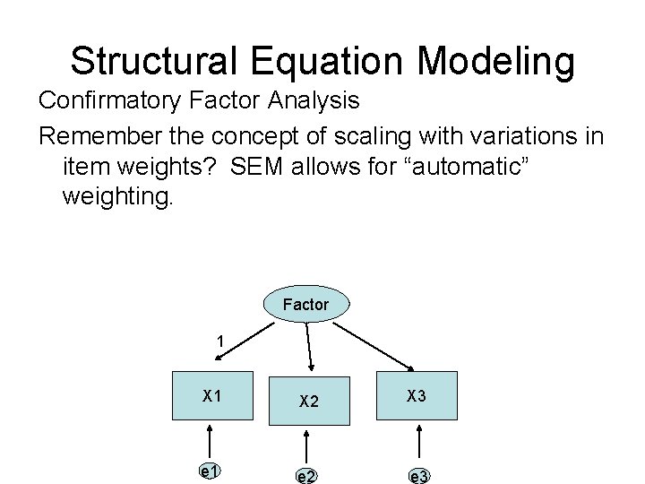
Structural Equation Modeling Confirmatory Factor Analysis Remember the concept of scaling with variations in item weights? SEM allows for “automatic” weighting. Factor 1 X 2 X 3 e 1 e 2 e 3

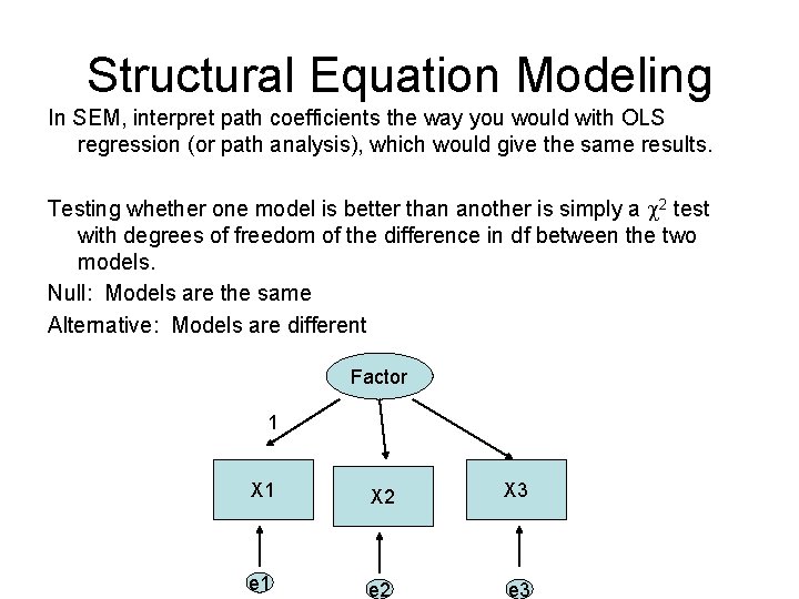
Structural Equation Modeling In SEM, interpret path coefficients the way you would with OLS regression (or path analysis), which would give the same results. Testing whether one model is better than another is simply a 2 test with degrees of freedom of the difference in df between the two models. Null: Models are the same Alternative: Models are different Factor 1 X 2 X 3 e 1 e 2 e 3

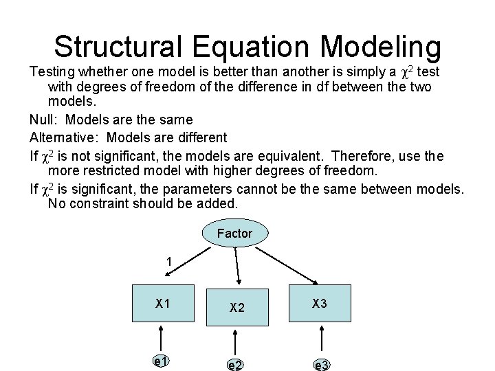
Structural Equation Modeling Testing whether one model is better than another is simply a 2 test with degrees of freedom of the difference in df between the two models. Null: Models are the same Alternative: Models are different If 2 is not significant, the models are equivalent. Therefore, use the more restricted model with higher degrees of freedom. If 2 is significant, the parameters cannot be the same between models. No constraint should be added. Factor 1 X 2 X 3 e 1 e 2 e 3

Structural Equation Modeling If 2 is not significant, the models are equivalent. Therefore, use the more restricted model with higher degrees of freedom. If 2 is significant, the parameters cannot be the same between models. No constraint should be added. This indicates a way to test whether two parameters are equal—just constrain them to be equal and compare the fit. Ways to test whether parameters are zero—just constrain them to be zero and compare the fit. Factor 1 X 2 X 3 e 1 e 2 e 3