Glaciation and the Pleistocene Over the last two

Glaciation and the Pleistocene

Over the last two million years, severe climatic changes had tremendous influence on life on earth. These events were recent enough that a number of techniques that they can be studied using techniques that are not available for more ancient times. Pleiostocene pack rat midden in eastern Nevada

Over its history, the earth has undergone many periods of extensive glaciation. Often, this resulted when plate movements positioned large continental blocks over the poles. Much of the Mesozoic and early Cenozoic, however, were characterized by mild climates. Therefore, the glacial and interglacial cycles of the Pleistocene represented a dramatic shift. The Wisconsin maximum

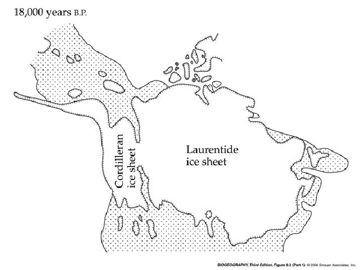
During the Pleistocene, the earth experienced numerous glacial-interglacial cycles. The glaciers were enormous, often 2 -3 km thick. At their maximum extent, they covered up to a third of the earths land surface. At the maximum extent of the last glacial period, ice sheets extended to about 45º N. latitude During the last glacial maximum (about 18, 000 years B. P. ) the Gulf Stream helped keep the North Atlantic relatively warm. It also cooled southern Europe and Africa as it flowed southward.

The last glacial maximum was largely (not entirely) a North American phenomenon.

During these glacial maxima, prevailing winds shifted. Moist air penetrated into the interior of most continents, causing wet (glacio-pluvial) conditions regions that are now arid. The same climate patterns led now moist tropical regions to be drier during glacial maxima. Glaciation was largely a northern hemisphere phenomenon, simply because of the distribution of land masses. Glacio-pluvial lakes of western North America

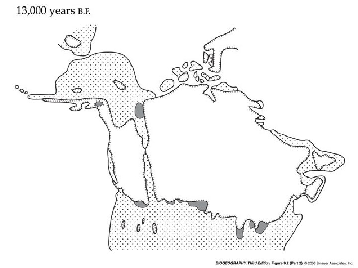
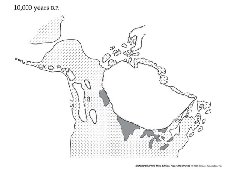
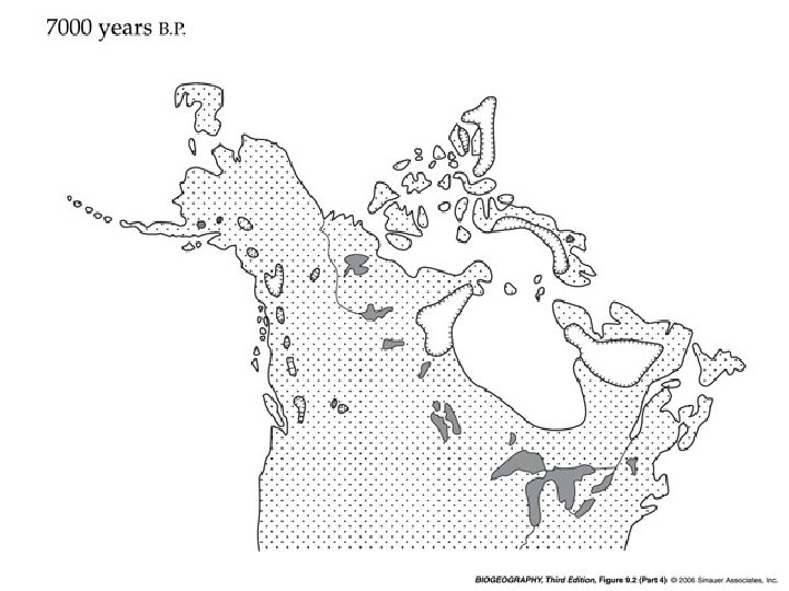
Move through the next few slides to examine the glacial recession in North America since the Wisconsin glaciation, the last glacial maximum of about 18, 000 B. P. (before present). Watch for: 1. The retreat of the Laurentide ice sheet, leaving the Great Lakes behind. 2. The opening of unglaciated areas between the Laurentide and the Cordilleran ice sheets. 3. The creation of massive Lake Agassiz, which will ultimately burst through the ice dam and empty into the forming Hudson Bay.

The “dumping” of Lake Agassiz is thought by some paleoclimatologists to have triggered the “Younger Dryas”. The present-day Minnesota River Valley was a drainage basin for Lake Agassiz.

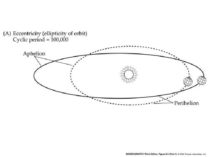
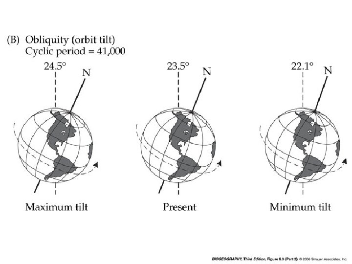
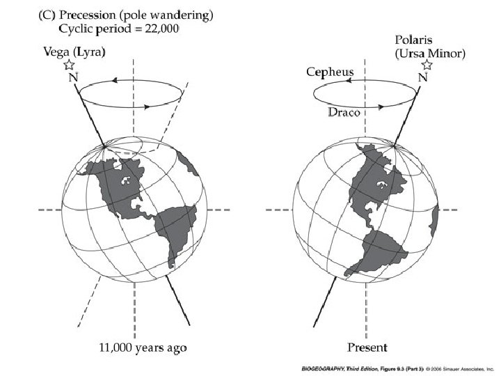
What caused the ice ages? Scientists once believed that they had resulted from changes in the output of solar radiation from the sun. This does not appear to be the case. Instead, the Pleistocene ice ages seem to have resulted from changes in the Earth’s orbit which, in turn, resulted in changes in incident solar radiation. These changes are known as Milanovitch cycles.

Milankovitch cycles are periodic changes in: 1. the eccentricity of the earth’s orbit, i. e. , how elliptical the orbit is. This occurs with a period of about 100, 000 years. 2. obliquity, i. e. the tilt of the earth’s axis to the plane of the ecliptic. This occurs with a period of about 41, 000 years, over which time the tilt changes from about 22. 1 to about 24. 5. The current tilt is about 23. 5. 3. The precession of the “point” of the poles. This occurs with a period of about 22, 000 years.

It’s also believed that, as ice developed, the increased albedo of the earth led to further cooling.

What’s the Evidence? By analyzing the oxygen contained in the Ca. CO 3 shells of preserved marine invertebrates, we can determine the amount of 16 O and 18 O present in the atmosphere at the time of the shell formation. The lighter 16 O evaporates more rapidly during warmer periods. With calibration, this ratio can be used to esimate temperatures.

Past and (predicted) future changes in the Milankovitch cycles. Periods of the cycles remain relatively constant, but their amplitude varies considerably.

Estimated average global air temperature over the past 850, 000 years (inferred from oxygen isotope) measurements from ice cores. Note that we are currently in a very warm interglacial period. In general, interglacials tend to be brief in duration. The earth has undergone at least twenty major glacial periods over the past 2 million years. If you’re wondering how these determinations can be made, here’s a link to a site that describes the use of oxygen ratios in paleoclimatology.

Records of global ocean temperatures over the last 140, 000 years indicate that the last two shifts from interglacials to glacial maxima took place of just a few thousand years.

Air temperatures from Eastern Europe over the last 10, 000 years….

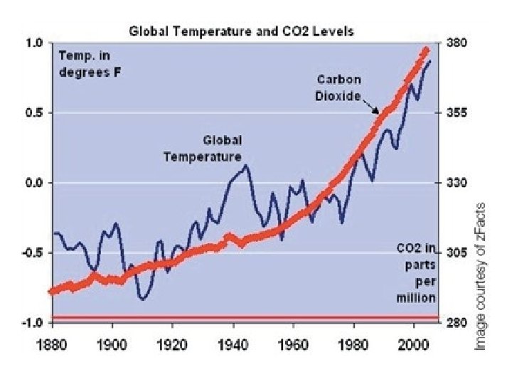
…and the variation in mid -latitude air temperatures from the Northern Hemisphere over the last thousand years. Again, note that the changes can be rapid. Global temperatures have varied significantly over the last millenium. After the relatively warm Middle Ages, temperatures cooled rapidly and we experienced the “Little Ice Ages”. A recent warming trend began about 150 years ago, and another cooling trend began around 1940.

This cooling trend seems to have been halted and reversed over the last twenty years, apparently by anthropogenicallyinduced warming.

During the Pleistocene, climates were influenced far south of the glaciers. This figure indicates that many unglaciated regions of North and South America were from 4 to 8 C. cooler in the Pleistocene than they are today.

The Laurentide ice sheet which existed from 18, 000 -9, 000 B. P. caused changes in prevailing wind patterns. This had great influence on local climates. While, globally, average ocean temperatures just dropped a couple of degrees, the temperature of the North Atlantic dropped as much as 10 C.

As winds moved down the very tall, steep faces of the glaciers, they warmed adiabatically. This moderated conditions in regions adjacent to the glaciers.

Sea Level Change

The lowering of sea level during the Pleistocene led to the formation of Beringia, which connected North America and Asia. These eustatic changes were global fluctuations in sea level that resulted from the freezing of massive quantities of water.

A better view of Beringia.

Lower sea level also resulted in the connection of many of the islands of Indonesia with the mainland of Asia and Australia, respectively. Wallace’s Line, a major biogeographic division, reflects the separation between those glacial land masses.

Two different methods have been used to estimate ancient sea levels, oxygen istope data and the depth of fossil coral reefs. Estimates derived from these two estimates agree reasonably well.

An examination of sea level changes throughout the Pleistocene reveal how rapidly (in a geological sense) the transition from glacial to interglacial conditions can occur.

The coastline of the southeastern U. S. has also changed dramatically since the last glacial maximum.

During the most recent glacial retreat, sea level rose rapidly, creating a shallow sea that covered the Saint Lawrence River Valley, Lake Champlain, and the Ottawa River.

A depiction of animals at the edge of the Champlain Sea. Many marine fossils have been found there, including a number of large marine mammals.

This explains the disjunct distribution of plants such as the seaside spurge, Euphorbia polygonifolia.

Biogeographic Responses to Glaciation A disjunct distribution

Biogeographic changes were triggered by three environmental changes that occurred as a result of the glacial/interglacial cycle. 1. Changes in the location, extent, and configuration of prime habitats. 2. Changes in the nature of climatic and environmental zones. 3. Formation and removal of dispersal routes.

The responses of biotas can also be placed into three categories. 1. Some species were able to move with their optimal habitat as it changed location. 2. Some species remained in place and adapted to new conditions. 3. Some species underwent range reductions, and many ultimately became extinct.

Vegetation zones in Europe during the last glacial maximum (Würm). The zones for most types were shifted to the south by 10 to 20 latitude. In some cases, eastwest mountain ranges blocked the southward range shift.

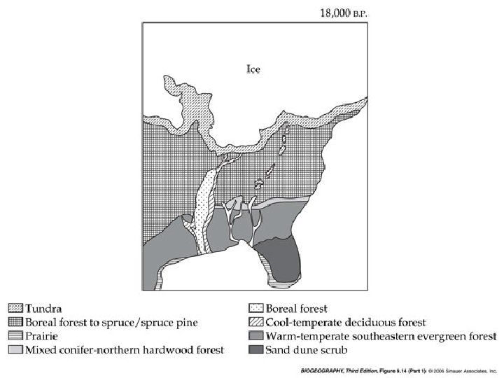
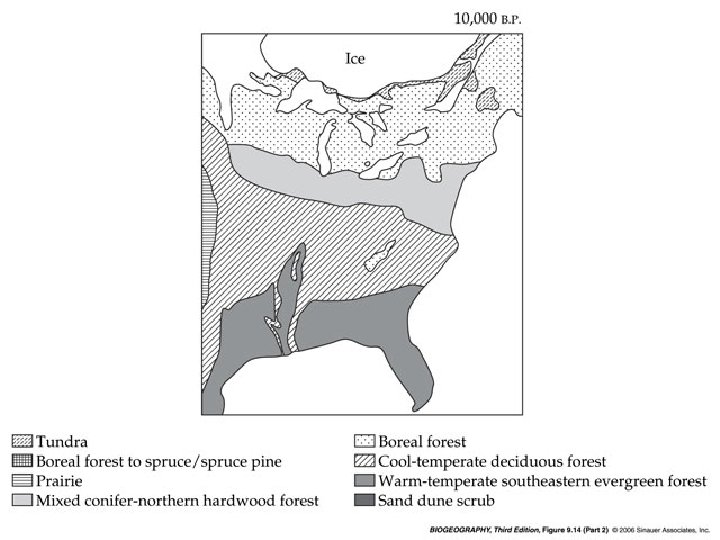
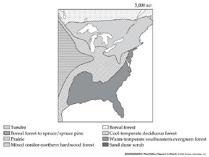
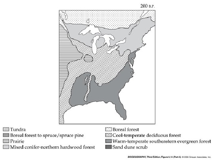
In contrast, the “north -south” mountain ranges and major rivers of North America made it easy for high latitude biomes to shift to the south. The next few slides show the gradual northward retreat of those biomes following the Wisconsin maximum of 18, 000 B. P.

Pollen profiles in the Andes Mountains of South America show vegetation zones have shifted upward since the last glacial maximum. Compare the illustrations below, showing the distribution of vegetation on Andean slopes at the time of the glacial maximum and today. The increasingly warm climate has forced the retreat of the cold-adapted vegetation found higher on the slopes. Note the upward shift of most vegetation zones. Realize how this elevation shift relates to the latitudinal shifts seen earlier.

And look at this…. These graphs represent the upper elevational limits of tropical forests (as determined from pollen analysis) in mountains of three different regions (East Africa, New Guinea, and South America) over the last 33, 000 years. Note that in these widely separated regions, the elevation of the tropical forest decreased from about 28, 000 B. P. to around 16, 000 B. P. , then began to increase. This represents the cooler climate of the glacial period (during which the forests shifted to lower elevation), followed by the warming of the interglacial with the concurrent upward shift of the forest.

We see dramatic latitudinal vegetation shifts in southern hemisphere regions as well. Note the dramatic changes in vegetation zones along the eastern coast of Australia. This shift from a dryadapted woodland to rain forest illustrates that the responses to glacial and interglacial conditions are not uniform.

The overall change in vegetation types in North America has been a dramatic decrease in tundra, with increases in deciduous forests, northern hardwoods, mixed forests, and coniferous forests.

Inland lodgepole pines have expanded their range northward over the last 12, 000 years. The northern range boundaries (as indicated by pollen records) at various dates before present are indicated by the dots.

The northward range expansion of the white spruce following the retreat of the Laurentide glacier was facilitated by prevailing winds (shown by the white arrows). After the range expansion had reached the edge of the glacier, the northerly winds aided in a rapid range expansion to the north.

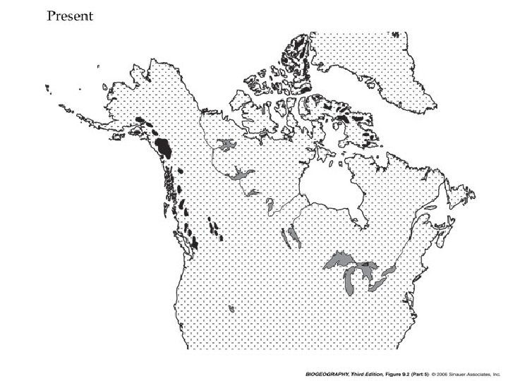
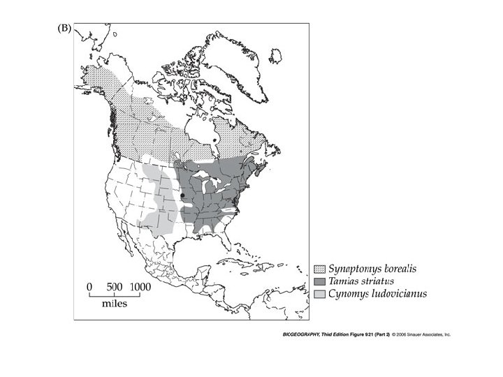
The next few slides illustrate the range shifts of four species of rodents during the Holocene. In each, the shaded area represents the present range, while the dots indicate the location of late Pleistocene fossils. The range shifts differ from species to species. The direction and length of the arrow indicate the magnitude and direction of the range shift. This one is the collared lemming (Dicrostonyx).

The range shift of the brown lemming (Lemmus) is smaller in magnitude.

The eastern chipmunk (Tamias striatus) shifted to the northeast.

The northern pocket gopher (Thomomys talpoides) shifted to the west.

How can we explain differences in the rate of range expansion of tree species following the recession of the glaciers?

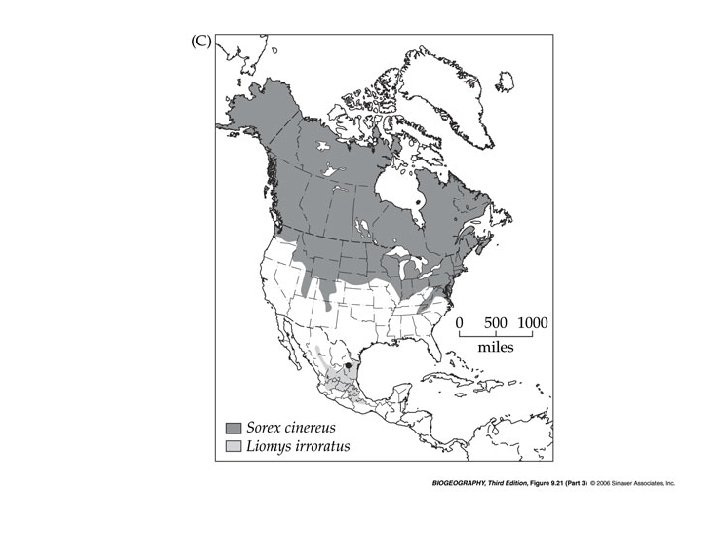
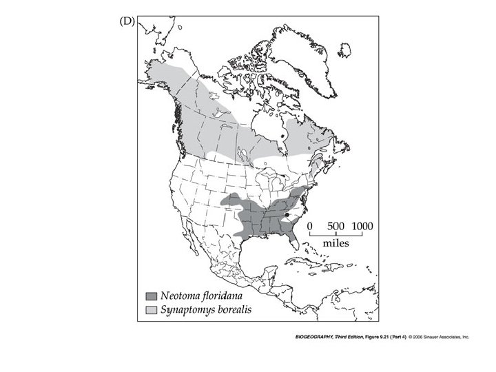
Differences in range shifts may have a number of results. In these cases, species which co-occurred during the most recent glacial maximum have become disjunct today. In these figures, current ranges of species are shown. The dot represents a location where late Pleistocene fossils of all are found together.

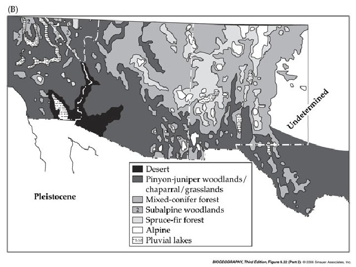
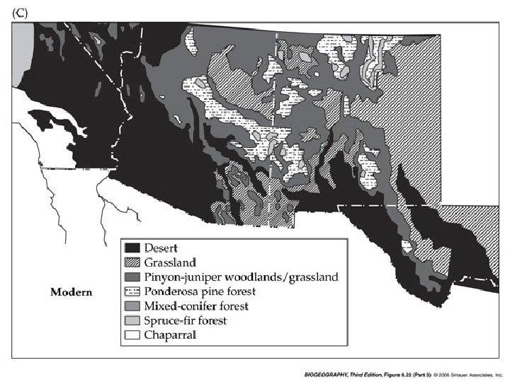
Significant changes in elevational distribution of vegetation have occurred since the Pleistocene. This is in the mountainous region of the American Southwest near southern Arizona. Notice that the elevational range was lower during the glacial periods of the Pleistocene.

The next two slides show the distribution of vegetation zones in the southwestern United States during the last glacial period compared with those today. By moving back and forth between the two slides, you can see that desert regions have expanded greatly, while vegetation zones adapted to cooler climates have declined. Alpine habitat has disappeared, while the coniferous forests that were widespread during the glacial period have declined dramatically.

Glacial Lake Agassiz covered much of present-day central Canada about 9000 B. P. About 8000 B. P. , the ice dam holding the waters behind it burst with a catastrophic release of fresh water into Hudson Bay.

Shyok Ice Lake is a modern-day example of a post-glacial lake formed when retreating glaciers served as dams and meltwater accumulated in glacier-carved valleys. Shyok is located along the western edge of the Himalayas.

Kettle lakes were formed when retreating glaciers left ice blocks behind on the outwash plain. Lakes formed in the outwash and in the glacial till by the melting blocks of ice.

A glacial plunge pool lake is formed when meltwater runs across the surface of the glacier and then pours down its face. A circular lake is carved at the foot of the glacial face.

Chapel Lake is one of several plunge pool lakes created by post glacial rivers after the Marquette advance of the most recent ice age. Its greatest depth is 140 feet.

Pluvial lakes were found across the western portion of North America during the Wisconsin glacial maximum. During the glacio-pluvial period, these areas experienced wetter conditions than the present. Most of what is now desert was then lakes and marshes. Massive Lake Bonneville has, today, been reduced to Great Salt Lake. The dissection of other pluvial lakes into smaller bodies of water has led to many instances of vicariant speciation. A wellstudied example of this occurred with the desert pupfish.

Haffer identfied six principal areas within the Amazon basin that are characterized by high endemicity. He proposed that these areas were refugia. He thought that they had remained as regions of rain forest during the glacial maxima, while the regions around them became more arid. Haffer and his colleagues felt that these regions were isolated during the glacial maxima, and that the isolation was long enough for significant speciation to take place. They felt that these speciation events explained, in part, the high diversity of the Amazon basin.

Regions receiving high rainfall were thought to have served as Pleistocene refugia. Patterns of distribution of some groups, like the toucanets illustrated above right, seemed to fall in line with this hypothesis.

Nunataks are refugia that persisted within or adjacent to the ice sheets. It appears that such ice-free areas might have existed between the Laurentide and Cordilleran ice sheets, and in a area of present-day southern Wisconsin known as the driftless refugium.

There may have also been icefree areas in mountainous regions along the Pacific Coast. These sites may have served as refugia, as well as acting as migration corridors during full glacial conditions.

This diagram represents the number or endemics in various regions of Alaska. The high frequency of endemic plant species in central Alaska (as many as 30 species in areas) suggests that much of Beringia remained unglaciated and served as a refugium for Arctic plant species during the Pleistocene.

In North America, mass extinctions of terrestrial vertebrates occurred during the late Pleistocene and early Holocene. Among the species that disappeared were mammoths, ground sloths, sabertooth cats, and giant bison.

Also going extinct were the giant teratorns vultures, shown here in comparison to modern condors.

Paul Martin proposed that the extinction of North American megafauna was the result of “overkill” by advancing human populations. This figures indicates the advance of human population in North America, beginning with the movement of humans across Beringia to colonize modern-day Alaska. They progressively moved to the south. As they moved, species of large mammals became extinct.

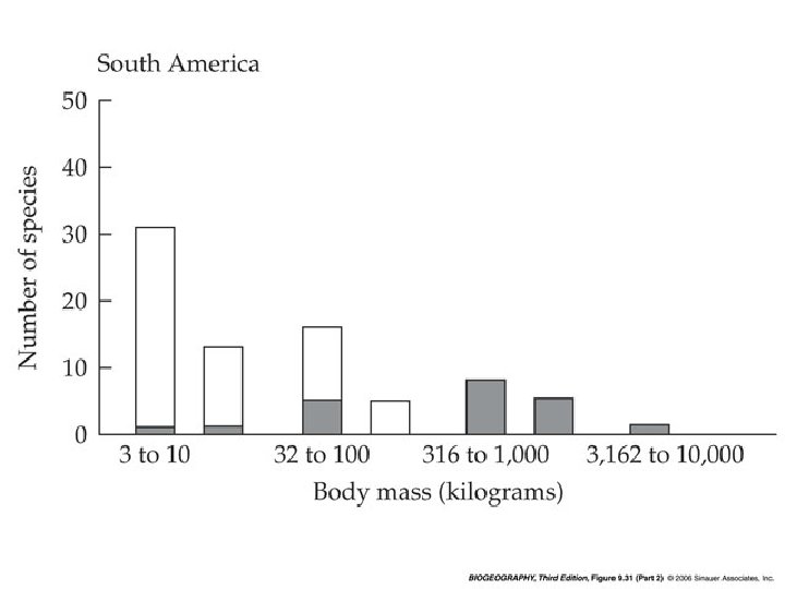
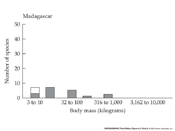
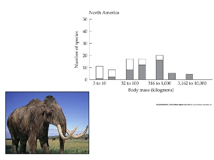
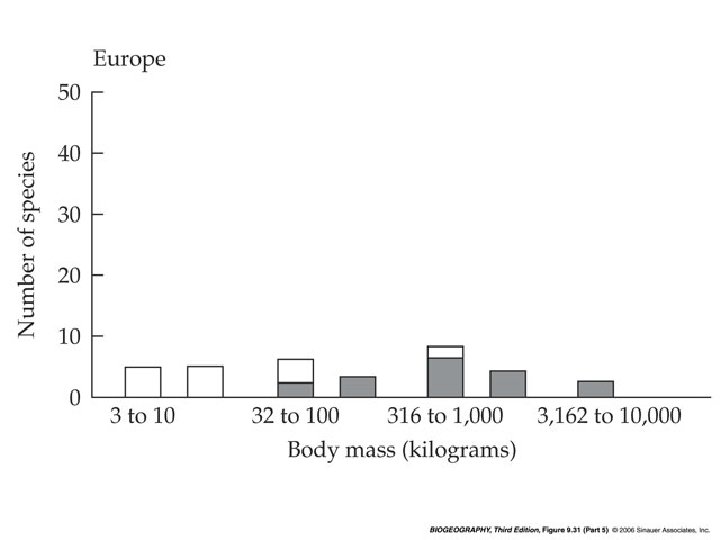
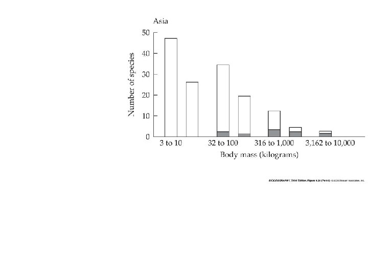
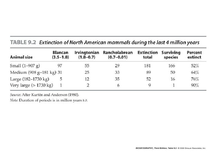
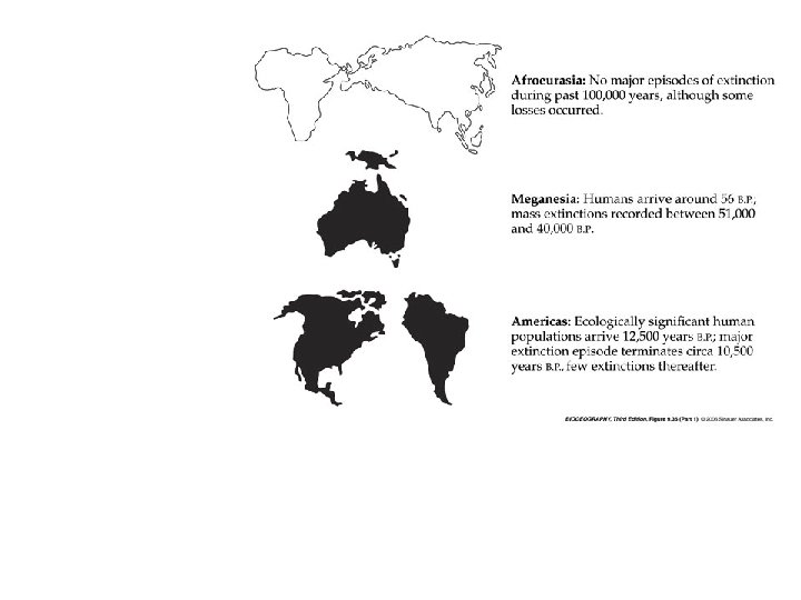
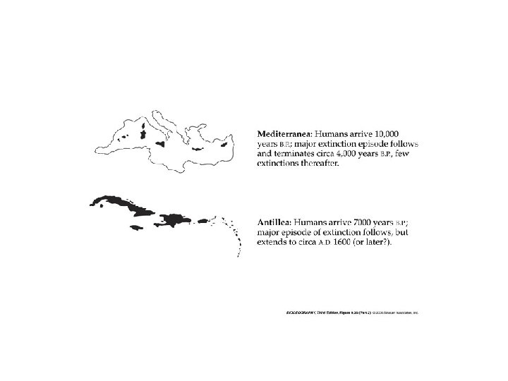
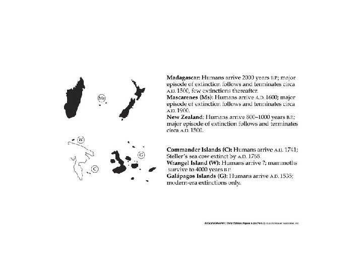
Quaternary extinctions were nonrandom. They varied significantly in timing from location to location, but always hit the largest taxa the hardest.

Geonynornis newtoni went extinct about 50 mya.

Africa is an exception, where the extinction of mammalian megafauna did not follow the same pattern. This may have been because the mammals of Africa evolved “with man”, and were not exposed as naïve prey to sophisticated Pleistocene hunters.

Extinction rates among moderately large herbivores during the late Pleistocene.

Are there alternative explanations for the Pleistocene extinctions? It does not appear that the late Pleistocene extinctions can be related directly to glaciation or any other catastrophic geological event, since the disappearance of North American megafauna did not take place until long after the retreat of the Wisconsin glaciers.

Extinction rates among native and immigrant large herbivores and carnivores in North America during the late Wisconsin. Immigrants did better than natives.

Selective extinctions of large megafaunal mammals in Australia after the arrival of humans. Species suffering extinction are shown in black. Those in gray became extinct after European colonization.