Chapter 6 Inverse Functions 6 1 Inverse Functions

Chapter 6 Inverse Functions

6. 1 Inverse Functions

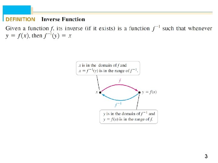
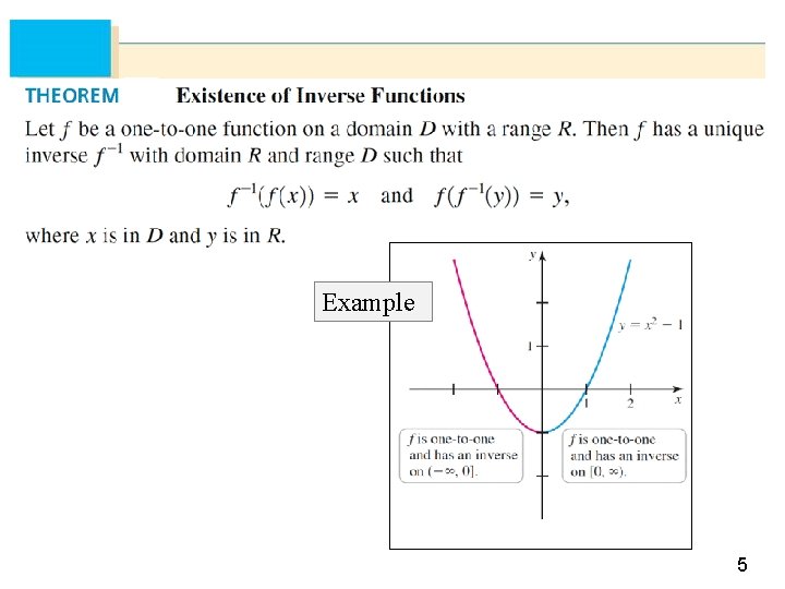
3

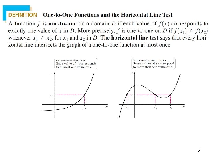
4

Example 5

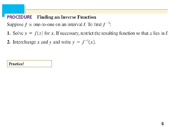
Practice! 6

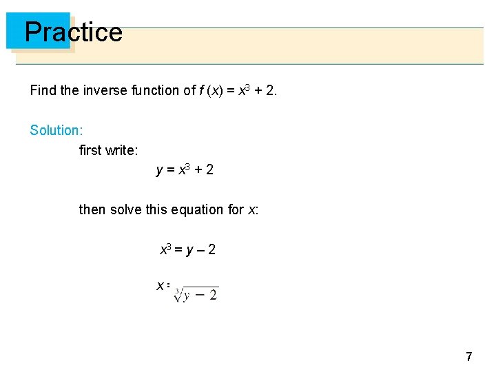
Practice Find the inverse function of f (x) = x 3 + 2. Solution: first write: y = x 3 + 2 then solve this equation for x: x 3 = y – 2 x= 7

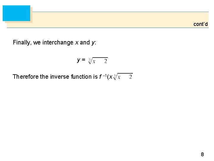
cont’d Finally, we interchange x and y: y= Therefore the inverse function is f – 1(x) = 8

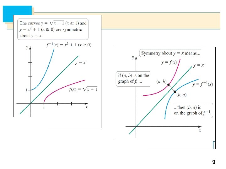
9

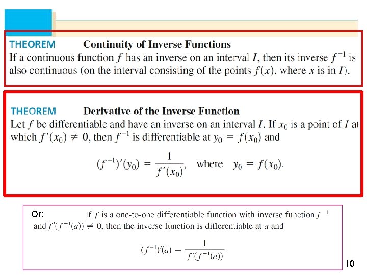
Or: 10

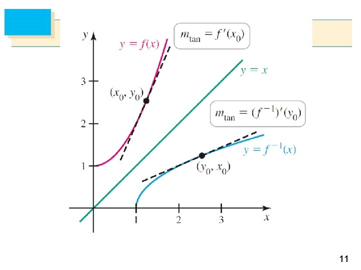
11

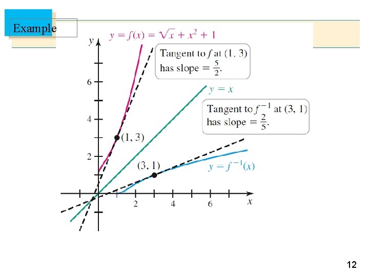
Example 12

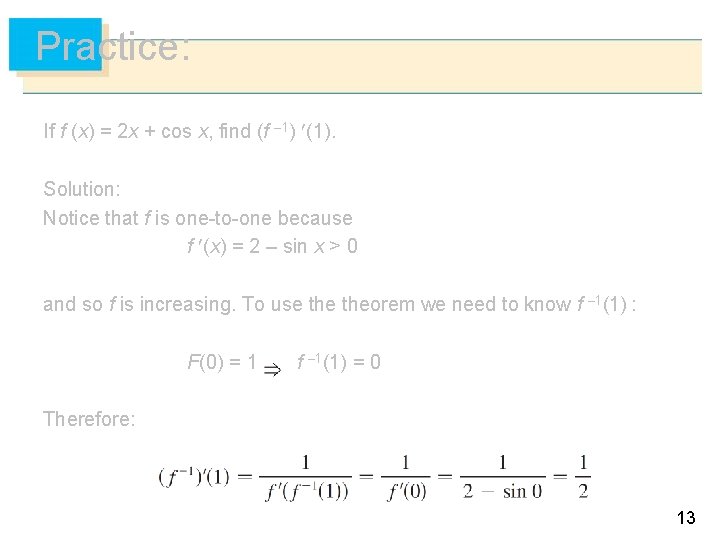
Practice: If f (x) = 2 x + cos x, find (f – 1) (1). Solution: Notice that f is one-to-one because f (x) = 2 – sin x > 0 and so f is increasing. To use theorem we need to know f – 1(1) : F(0) = 1 f – 1(1) = 0 Therefore: 13

6. 2 Exponential Functions

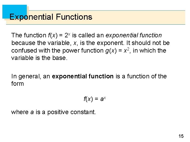
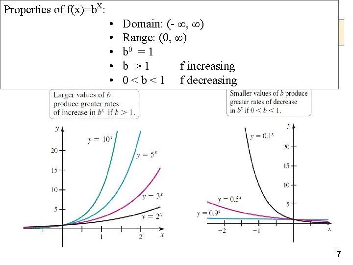
Exponential Functions The function f (x) = 2 x is called an exponential function because the variable, x, is the exponent. It should not be confused with the power function g (x) = x 2, in which the variable is the base. In general, an exponential function is a function of the form f (x) = ax where a is a positive constant. 15

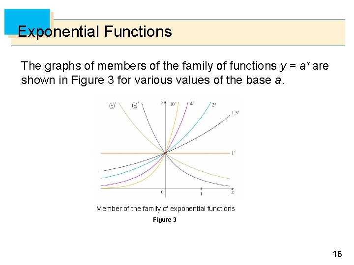
Exponential Functions The graphs of members of the family of functions y = ax are shown in Figure 3 for various values of the base a. Member of the family of exponential functions Figure 3 16

Properties of f(x)=bx: • • • Domain: (- ∞, ∞) Range: (0, ∞) b 0 = 1 b >1 f increasing 0 < b < 1 f decreasing 17

Exponential Functions Notice that all of these graphs pass through the same point (0, 1) because b 0 = 1 for b ≠ 0. Notice also that as the base b gets larger, the exponential function grows more rapidly (for x > 0). 18

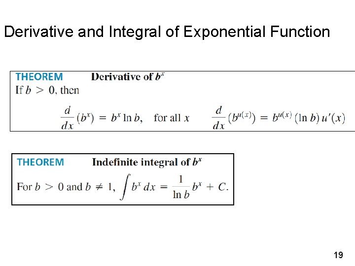
Derivative and Integral of Exponential Function 19

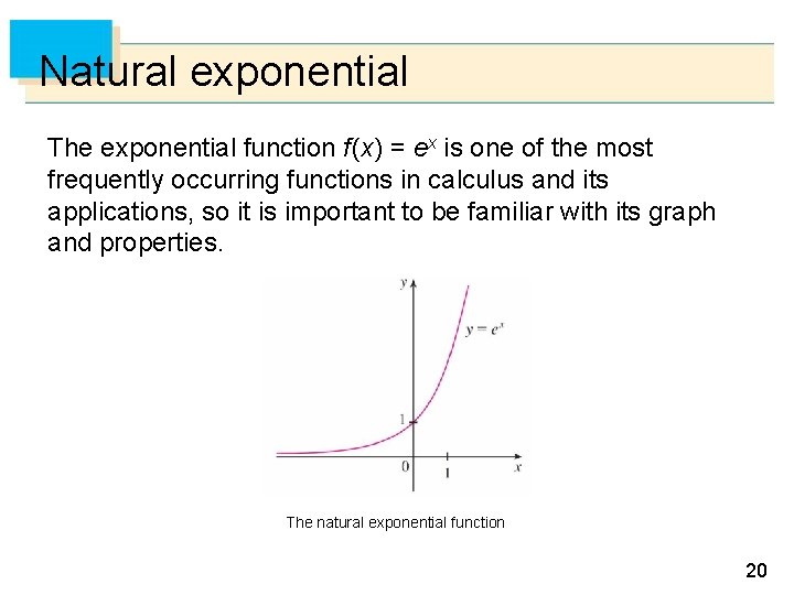
Natural exponential The exponential function f (x) = ex is one of the most frequently occurring functions in calculus and its applications, so it is important to be familiar with its graph and properties. The natural exponential function 20

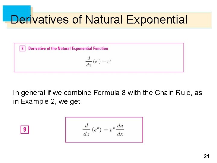
Derivatives of Natural Exponential In general if we combine Formula 8 with the Chain Rule, as in Example 2, we get 21

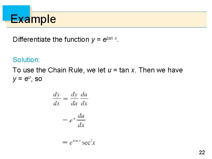
Example Differentiate the function y = etan x. Solution: To use the Chain Rule, we let u = tan x. Then we have y = eu, so 22

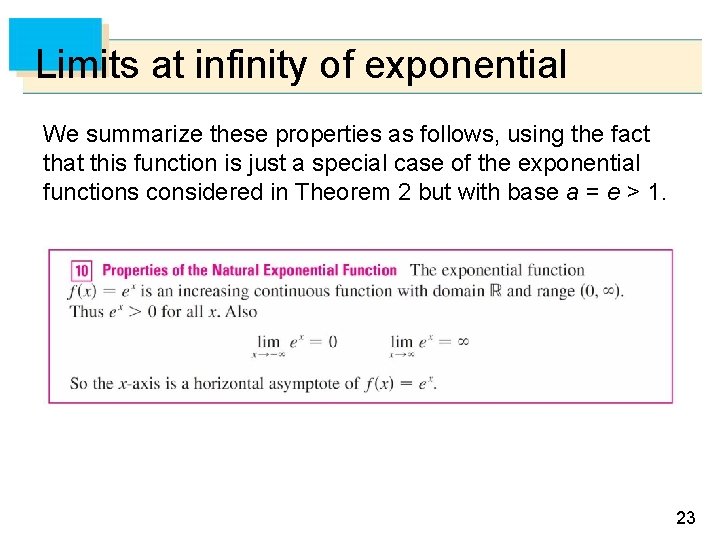
Limits at infinity of exponential We summarize these properties as follows, using the fact that this function is just a special case of the exponential functions considered in Theorem 2 but with base a = e > 1. 23

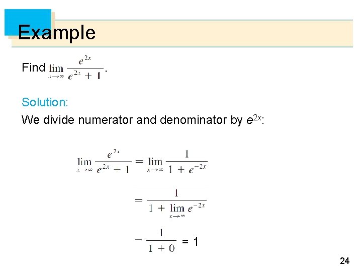
Example Find Solution: We divide numerator and denominator by e 2 x: =1 24

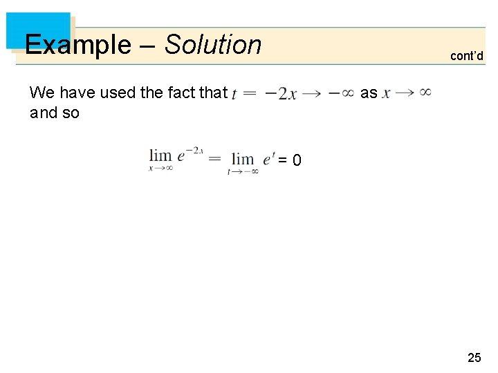
Example – Solution cont’d We have used the fact that and so as =0 25

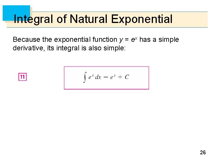
Integral of Natural Exponential Because the exponential function y = ex has a simple derivative, its integral is also simple: 26

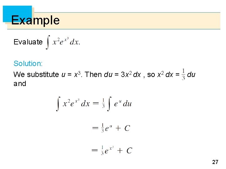
Example Evaluate Solution: We substitute u = x 3. Then du = 3 x 2 dx , so x 2 dx = du and 27

Applications of Exponential Functions 28

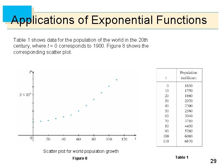
Applications of Exponential Functions Table 1 shows data for the population of the world in the 20 th century, where t = 0 corresponds to 1900. Figure 8 shows the corresponding scatter plot. Scatter plot for world population growth Figure 8 Table 1 29

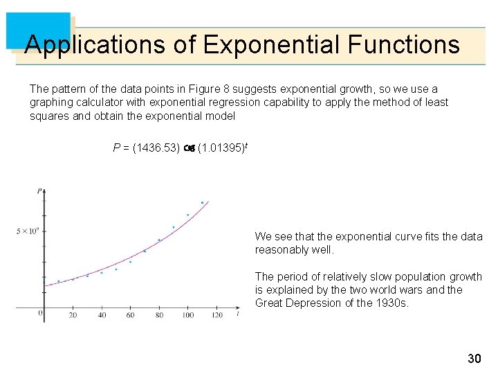
Applications of Exponential Functions The pattern of the data points in Figure 8 suggests exponential growth, so we use a graphing calculator with exponential regression capability to apply the method of least squares and obtain the exponential model P = (1436. 53) (1. 01395)t We see that the exponential curve fits the data reasonably well. The period of relatively slow population growth is explained by the two world wars and the Great Depression of the 1930 s. 30

6. 3 Logarithmic Functions 31

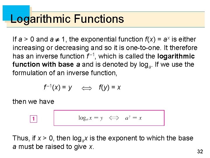
Logarithmic Functions If a > 0 and a 1, the exponential function f (x) = ax is either increasing or decreasing and so it is one-to-one. It therefore has an inverse function f – 1, which is called the logarithmic function with base a and is denoted by loga. If we use the formulation of an inverse function, f – 1 (x) = y f (y) = x then we have Thus, if x > 0, then logax is the exponent to which the base a must be raised to give x. 32

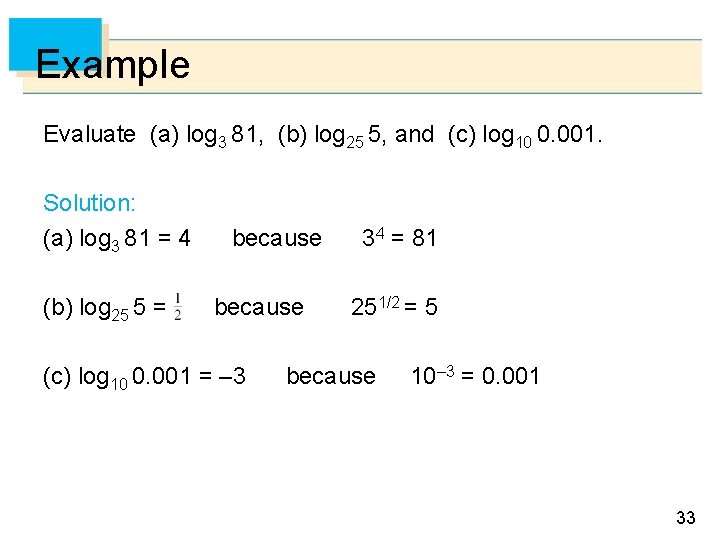
Example Evaluate (a) log 3 81, (b) log 25 5, and (c) log 10 0. 001. Solution: (a) log 3 81 = 4 (b) log 25 5 = because (c) log 10 0. 001 = – 3 34 = 81 251/2 = 5 because 10– 3 = 0. 001 33

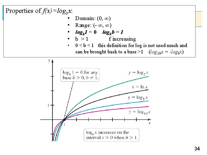
Properties of f(x)=logbx: • • Domain: (0, ∞) Range: (- ∞, ∞) logb 1 = 0 logbb = 1 b >1 f increasing • 0 < b < 1 this definition for log is not used much and can be brought back to a base >1 (log 1/bx = -logbx) 34

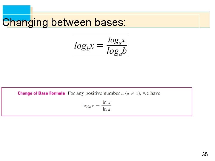
Changing between bases: 35

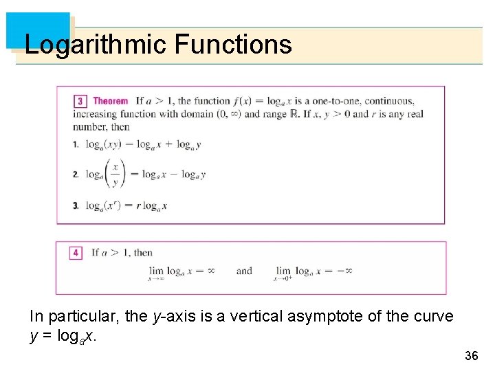
Logarithmic Functions In particular, the y-axis is a vertical asymptote of the curve y = logax. 36

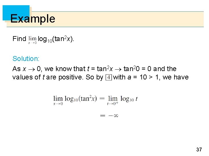
Example Find log 10(tan 2 x). Solution: As x 0, we know that t = tan 2 x tan 20 = 0 and the values of t are positive. So by with a = 10 > 1, we have 37

Natural Logarithms 38

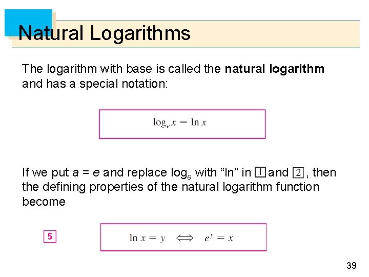
Natural Logarithms The logarithm with base is called the natural logarithm and has a special notation: If we put a = e and replace loge with “ln” in and , then the defining properties of the natural logarithm function become 39

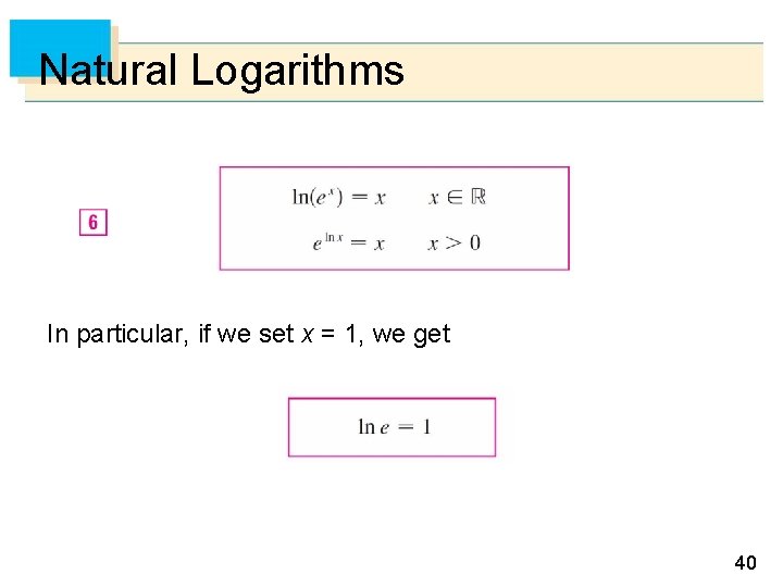
Natural Logarithms In particular, if we set x = 1, we get 40

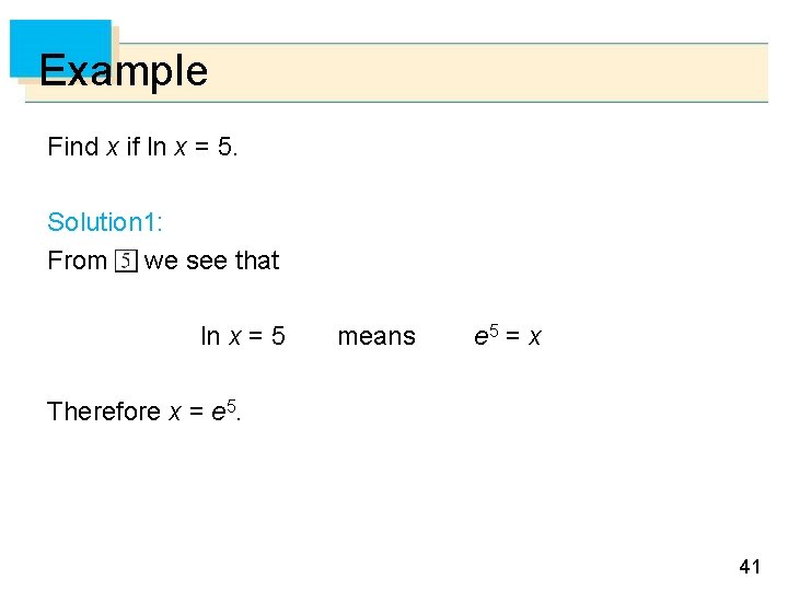
Example Find x if ln x = 5. Solution 1: From we see that ln x = 5 means e 5 = x Therefore x = e 5. 41

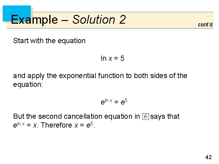
Example – Solution 2 cont’d Start with the equation ln x = 5 and apply the exponential function to both sides of the equation: eln x = e 5 But the second cancellation equation in eln x = x. Therefore x = e 5. says that 42

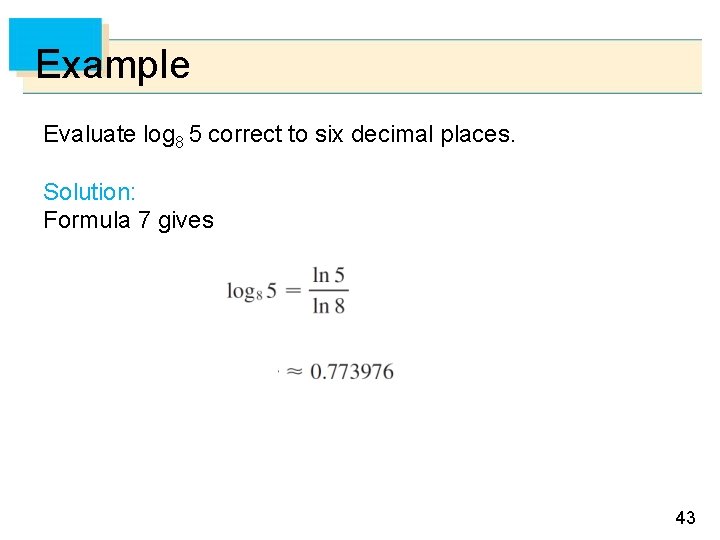
Example Evaluate log 8 5 correct to six decimal places. Solution: Formula 7 gives 43

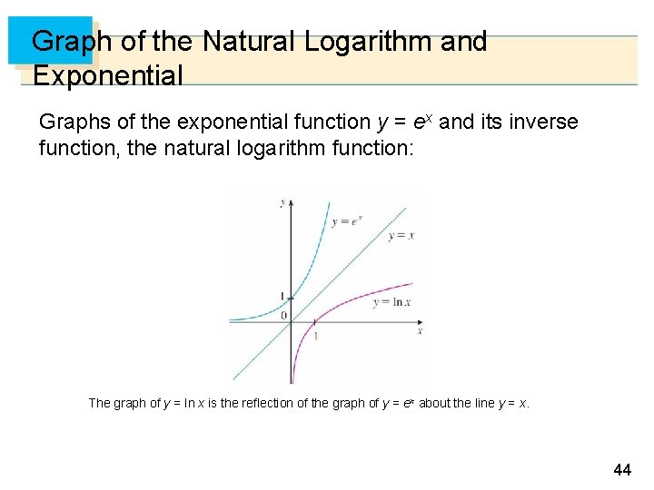
Graph of the Natural Logarithm and Exponential Graphs of the exponential function y = ex and its inverse function, the natural logarithm function: The graph of y = ln x is the reflection of the graph of y = ex about the line y = x. 44

6. 4 Derivatives of Logarithmic Functions 45

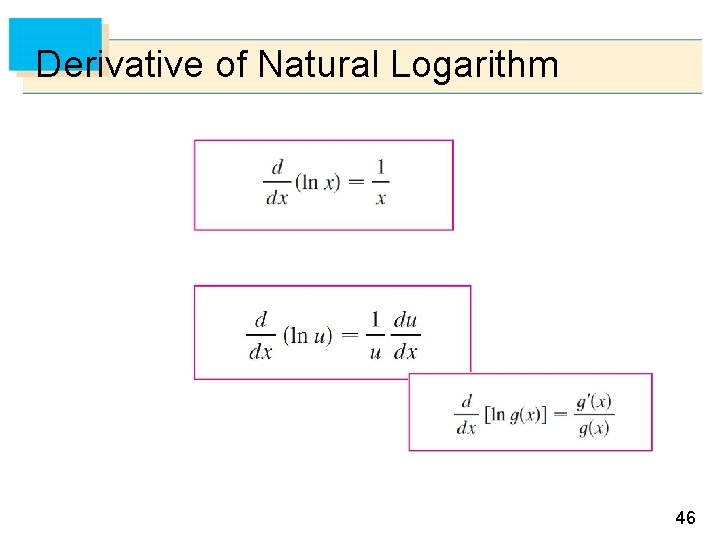
Derivative of Natural Logarithm 46

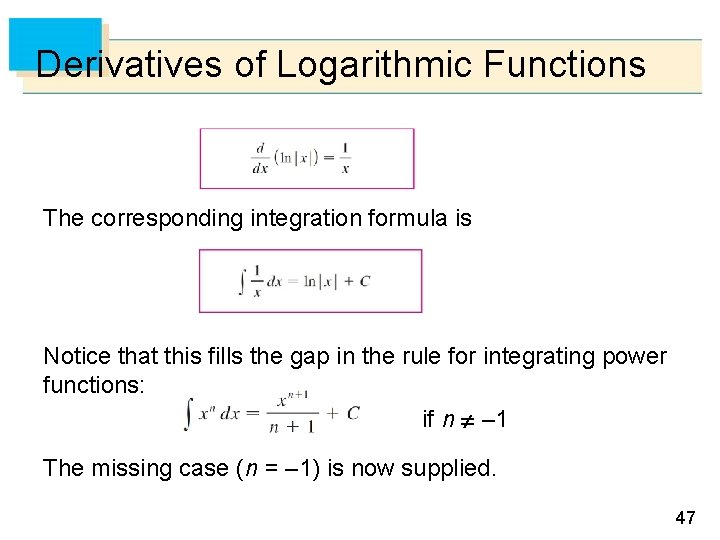
Derivatives of Logarithmic Functions The corresponding integration formula is Notice that this fills the gap in the rule for integrating power functions: if n – 1 The missing case (n = – 1) is now supplied. 47

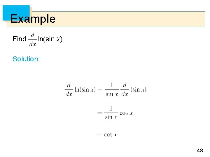
Example Find ln(sin x). Solution: 48

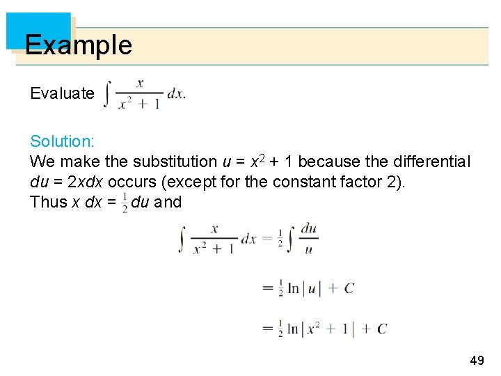
Example Evaluate Solution: We make the substitution u = x 2 + 1 because the differential du = 2 xdx occurs (except for the constant factor 2). Thus x dx = du and 49

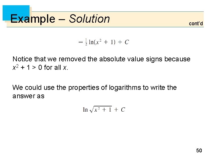
Example – Solution cont’d Notice that we removed the absolute value signs because x 2 + 1 > 0 for all x. We could use the properties of logarithms to write the answer as 50

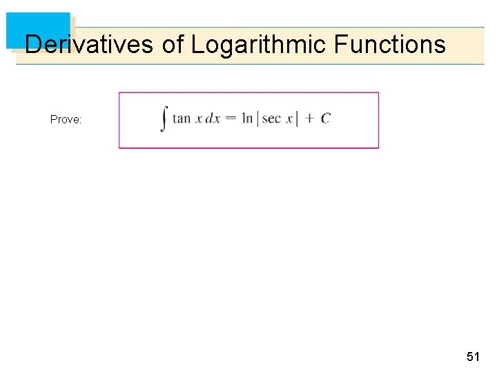
Derivatives of Logarithmic Functions Prove: 51

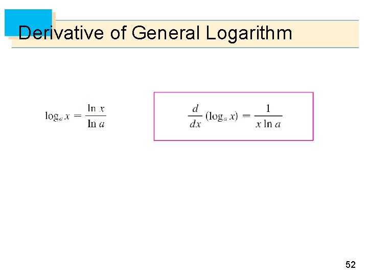
Derivative of General Logarithm 52

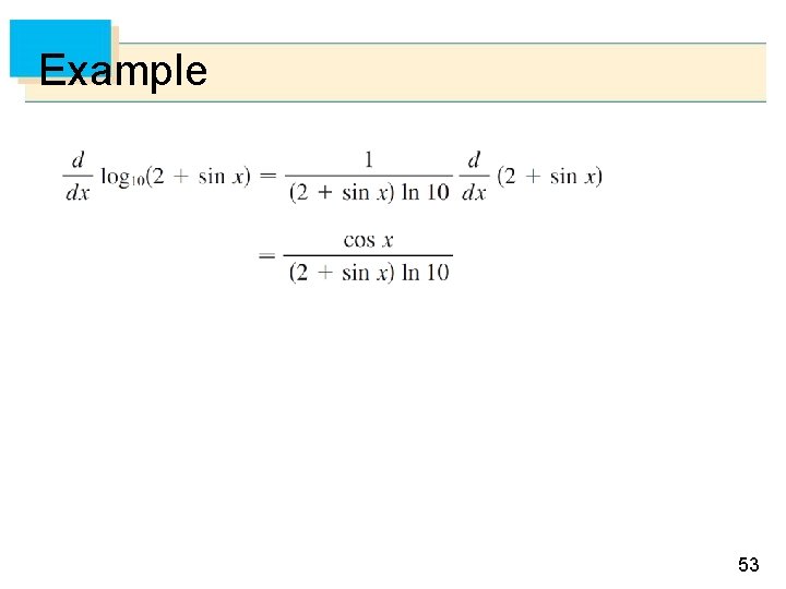
Example 53

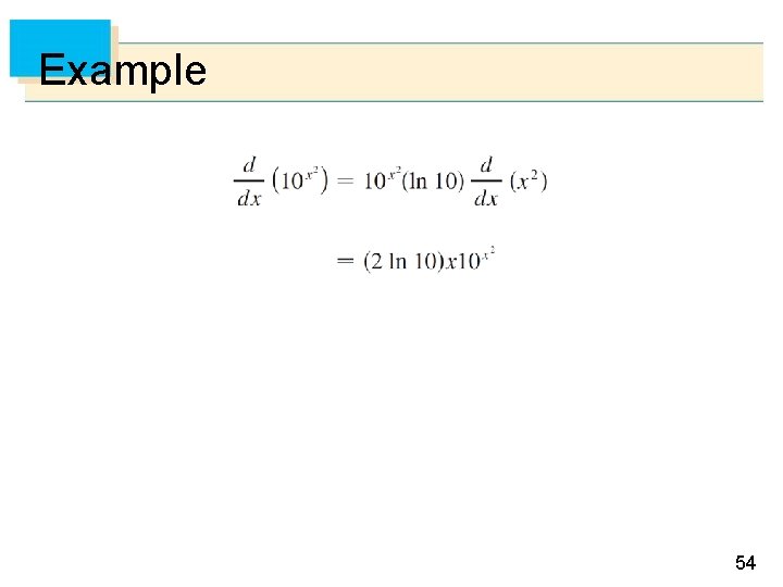
Example 54

Logarithmic Differentiation 55

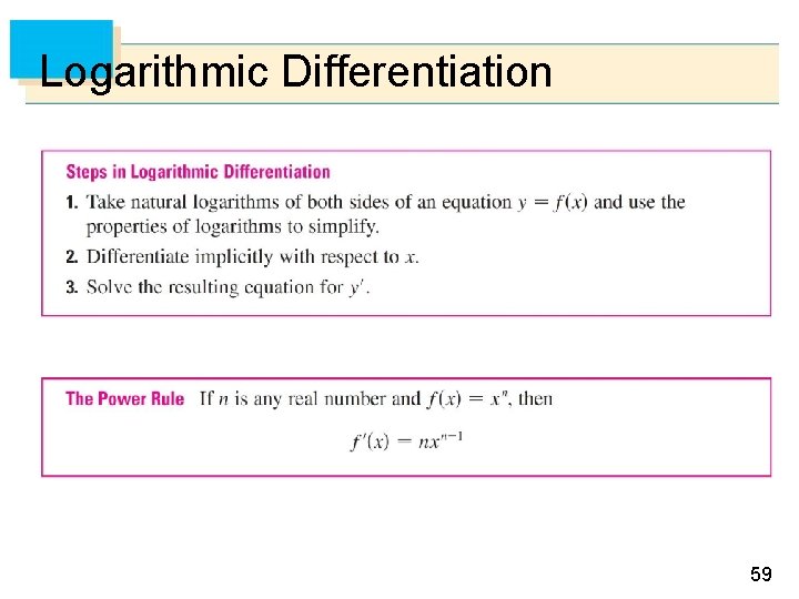
Logarithmic Differentiation The calculation of derivatives of complicated functions involving products, quotients, or powers can often be simplified by taking logarithms. The method used in the next example is called logarithmic differentiation. 56

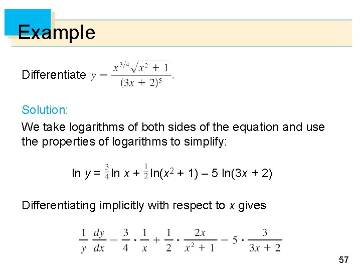
Example Differentiate Solution: We take logarithms of both sides of the equation and use the properties of logarithms to simplify: ln y = ln x + ln(x 2 + 1) – 5 ln(3 x + 2) Differentiating implicitly with respect to x gives 57

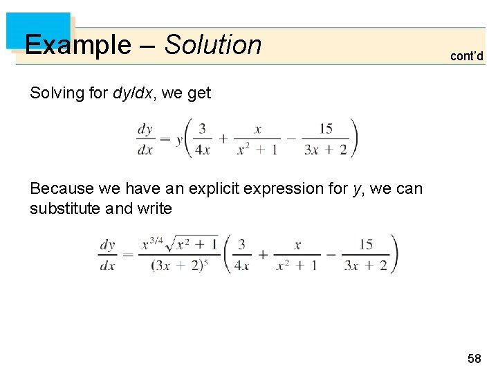
Example – Solution cont’d Solving for dy/dx, we get Because we have an explicit expression for y, we can substitute and write 58

Logarithmic Differentiation 59

6. 5 Exponential Growth and Decay 60

Exponential Growth and Decay In many natural phenomena, quantities grow or decay at a rate proportional to their size. For instance, if y = f (t) is the number of individuals in a population of animals or bacteria at time t, then it seems reasonable to expect that the rate of growth f (t) is proportional to the population f (t); that is, f (t) = kf (t) for some constant k. Indeed, under ideal conditions (unlimited environment, adequate nutrition, immunity to disease) the mathematical model given by the equation f (t) = kf (t) predicts what actually happens fairly accurately. 61

Exponential Growth and Decay Another example occurs in nuclear physics where the mass of a radioactive substance decays at a rate proportional to the mass. In chemistry, the rate of a unimolecular first-order reaction is proportional to the concentration of the substance. In finance, the value of a savings account with continuously compounded interest increases at a rate proportional to that value. 62

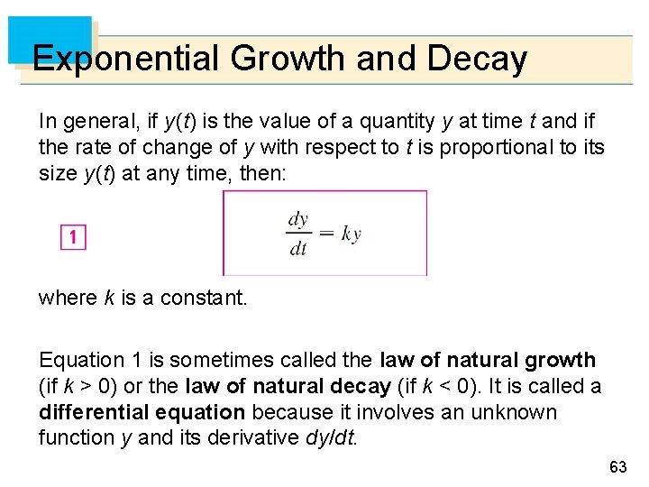
Exponential Growth and Decay In general, if y (t) is the value of a quantity y at time t and if the rate of change of y with respect to t is proportional to its size y (t) at any time, then: where k is a constant. Equation 1 is sometimes called the law of natural growth (if k > 0) or the law of natural decay (if k < 0). It is called a differential equation because it involves an unknown function y and its derivative dy/dt. 63

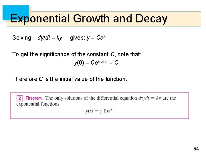
Exponential Growth and Decay Solving: dy/dt = ky gives: y = Cekt. To get the significance of the constant C, note that: y(0) = Cek 0 = C Therefore C is the initial value of the function. 64

Population Growth 65

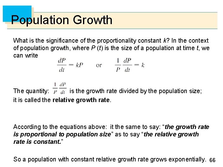
Population Growth What is the significance of the proportionality constant k? In the context of population growth, where P (t) is the size of a population at time t, we can write The quantity: is the growth rate divided by the population size; it is called the relative growth rate. According to the equations above: it the same to say: “the growth rate is proportional to population size” as to say “the relative growth rate is constant. ” So a population with constant relative growth rate grows exponentially. 66

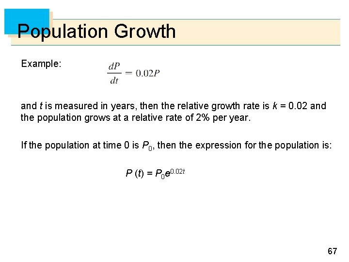
Population Growth Example: and t is measured in years, then the relative growth rate is k = 0. 02 and the population grows at a relative rate of 2% per year. If the population at time 0 is P 0, then the expression for the population is: P (t) = P 0 e 0. 02 t 67

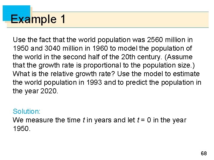
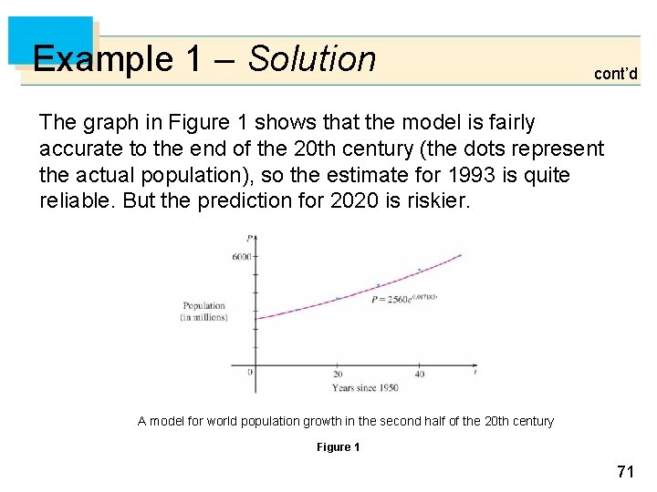
Example 1 Use the fact that the world population was 2560 million in 1950 and 3040 million in 1960 to model the population of the world in the second half of the 20 th century. (Assume that the growth rate is proportional to the population size. ) What is the relative growth rate? Use the model to estimate the world population in 1993 and to predict the population in the year 2020. Solution: We measure the time t in years and let t = 0 in the year 1950. 68

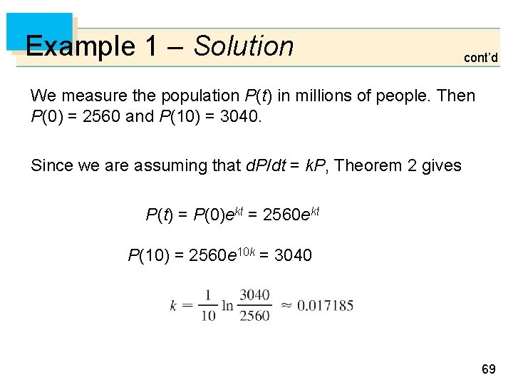
Example 1 – Solution cont’d We measure the population P(t) in millions of people. Then P(0) = 2560 and P(10) = 3040. Since we are assuming that d. P/dt = k. P, Theorem 2 gives P(t) = P(0)ekt = 2560 ekt P(10) = 2560 e 10 k = 3040 69

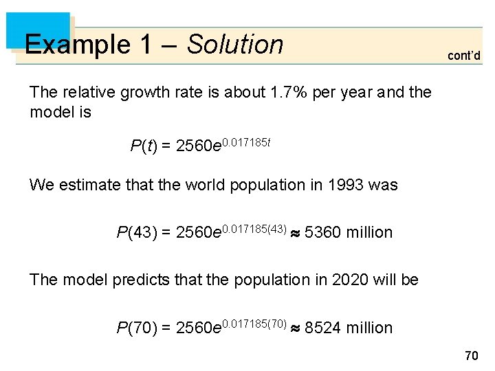
Example 1 – Solution cont’d The relative growth rate is about 1. 7% per year and the model is P(t) = 2560 e 0. 017185 t We estimate that the world population in 1993 was P(43) = 2560 e 0. 017185(43) 5360 million The model predicts that the population in 2020 will be P(70) = 2560 e 0. 017185(70) 8524 million 70

Example 1 – Solution cont’d The graph in Figure 1 shows that the model is fairly accurate to the end of the 20 th century (the dots represent the actual population), so the estimate for 1993 is quite reliable. But the prediction for 2020 is riskier. A model for world population growth in the second half of the 20 th century Figure 1 71

Radioactive Decay 72

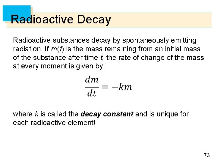
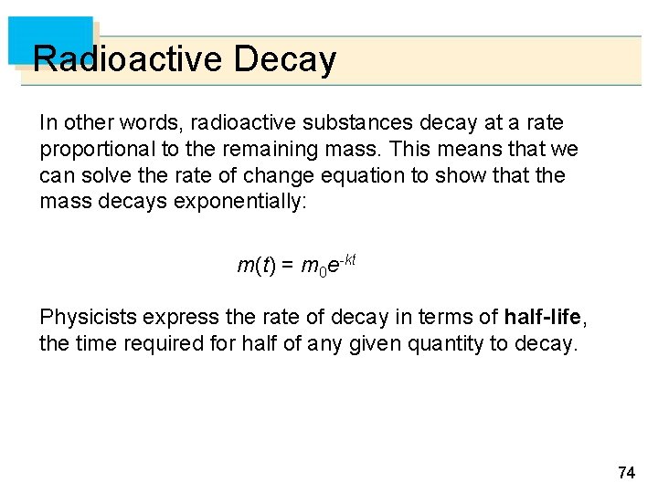
Radioactive Decay Radioactive substances decay by spontaneously emitting radiation. If m (t) is the mass remaining from an initial mass of the substance after time t, the rate of change of the mass at every moment is given by: where k is called the decay constant and is unique for each radioactive element! 73

Radioactive Decay In other words, radioactive substances decay at a rate proportional to the remaining mass. This means that we can solve the rate of change equation to show that the mass decays exponentially: m(t) = m 0 e-kt Physicists express the rate of decay in terms of half-life, the time required for half of any given quantity to decay. 74

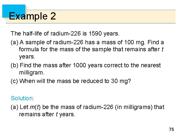
Example 2 The half-life of radium-226 is 1590 years. (a) A sample of radium-226 has a mass of 100 mg. Find a formula for the mass of the sample that remains after t years. (b) Find the mass after 1000 years correct to the nearest milligram. (c) When will the mass be reduced to 30 mg? Solution: (a) Let m(t) be the mass of radium-226 (in milligrams) that remains after t years. 75

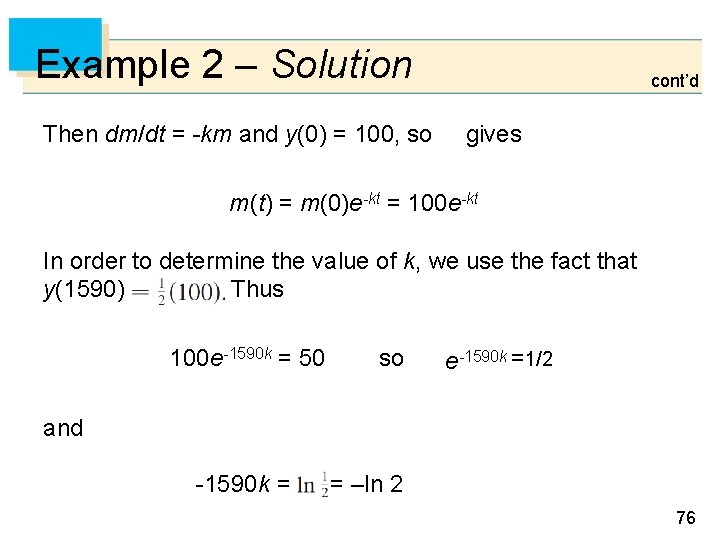
Example 2 – Solution Then dm/dt = -km and y(0) = 100, so cont’d gives m(t) = m(0)e-kt = 100 e-kt In order to determine the value of k, we use the fact that y(1590) Thus 100 e-1590 k = 50 so e-1590 k =1/2 and -1590 k = = –ln 2 76

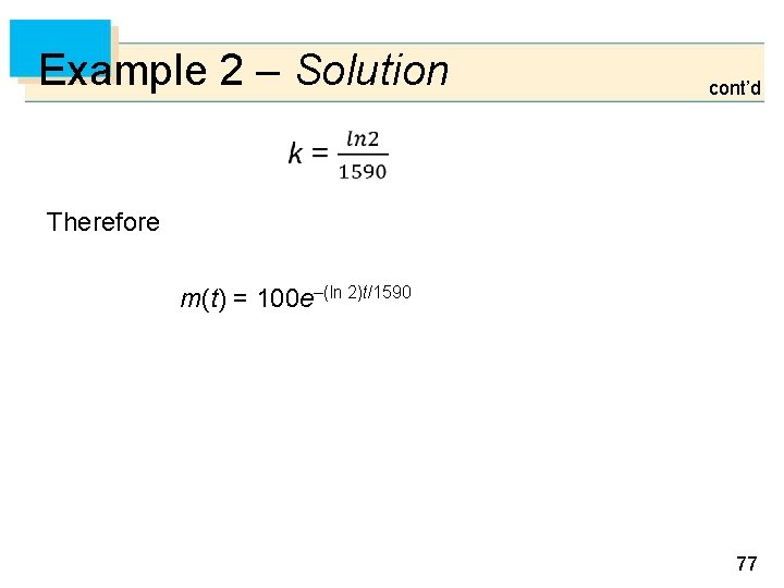
Example 2 – Solution cont’d Therefore m(t) = 100 e–(ln 2)t/1590 77

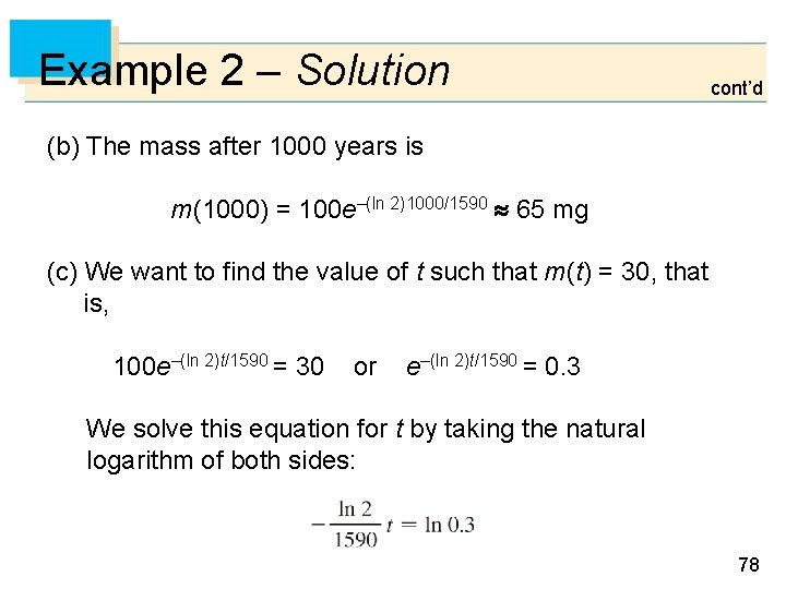
Example 2 – Solution cont’d (b) The mass after 1000 years is m(1000) = 100 e–(ln 2)1000/1590 65 mg (c) We want to find the value of t such that m (t) = 30, that is, 100 e–(ln 2)t/1590 = 30 or e–(ln 2)t/1590 = 0. 3 We solve this equation for t by taking the natural logarithm of both sides: 78

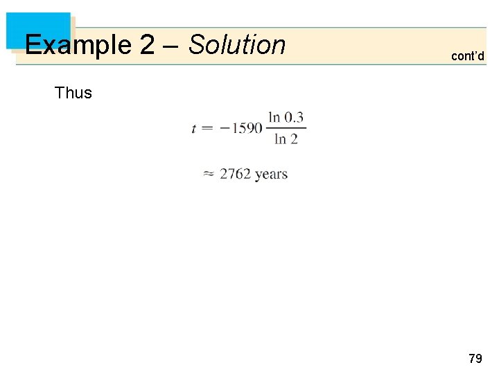
Example 2 – Solution cont’d Thus 79

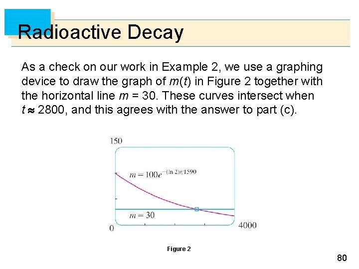
Radioactive Decay As a check on our work in Example 2, we use a graphing device to draw the graph of m (t) in Figure 2 together with the horizontal line m = 30. These curves intersect when t 2800, and this agrees with the answer to part (c). Figure 2 80

Newton’s Law of Cooling 81

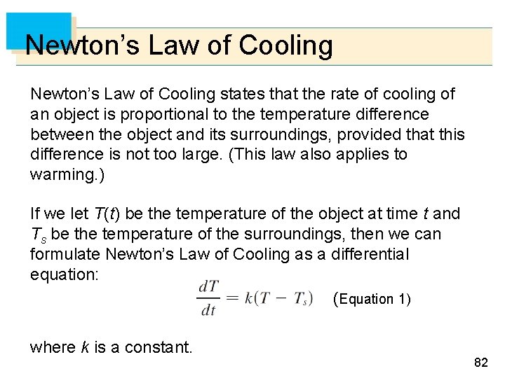
Newton’s Law of Cooling states that the rate of cooling of an object is proportional to the temperature difference between the object and its surroundings, provided that this difference is not too large. (This law also applies to warming. ) If we let T (t) be the temperature of the object at time t and Ts be the temperature of the surroundings, then we can formulate Newton’s Law of Cooling as a differential equation: (Equation 1) where k is a constant. 82

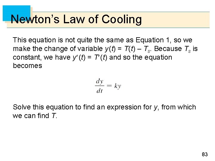
Newton’s Law of Cooling This equation is not quite the same as Equation 1, so we make the change of variable y (t) = T (t) – Ts. Because Ts is constant, we have y (t) = T (t) and so the equation becomes Solve this equation to find an expression for y, from which we can find T. 83

Example 3 A bottle of soda pop at room temperature (72 F) is placed in a refrigerator where the temperature is 44 F. After half an hour the soda pop has cooled to 61 F. (a) What is the temperature of the soda pop after another half hour? (b) How long does it take for the soda pop to cool to 50 F? Solution: (a) Let T (t) be the temperature of the soda after t minutes. 84

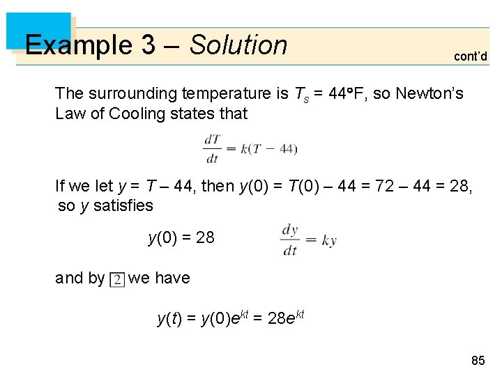
Example 3 – Solution cont’d The surrounding temperature is Ts = 44 F, so Newton’s Law of Cooling states that If we let y = T – 44, then y (0) = T (0) – 44 = 72 – 44 = 28, so y satisfies y (0) = 28 and by we have y (t) = y (0)ekt = 28 ekt 85

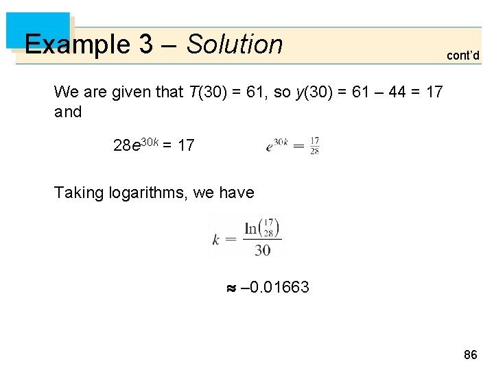
Example 3 – Solution cont’d We are given that T(30) = 61, so y(30) = 61 – 44 = 17 and 28 e 30 k = 17 Taking logarithms, we have – 0. 01663 86

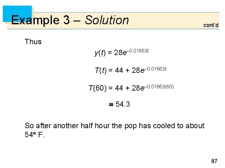
Example 3 – Solution cont’d Thus y(t) = 28 e– 0. 01663 t T(t) = 44 + 28 e– 0. 01663 t T(60) = 44 + 28 e– 0. 01663(60) 54. 3 So after another half hour the pop has cooled to about 54 F. 87

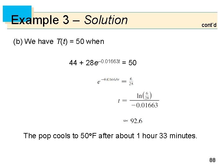
Example 3 – Solution cont’d (b) We have T(t) = 50 when 44 + 28 e– 0. 01663 t = 50 The pop cools to 50 F after about 1 hour 33 minutes. 88

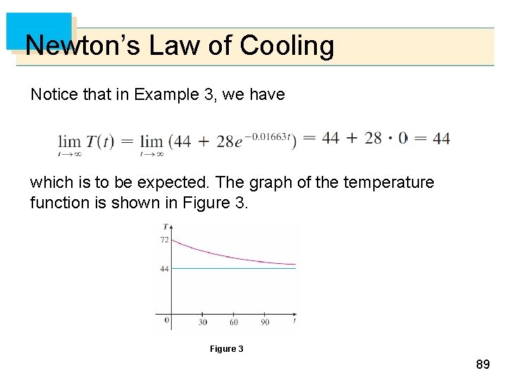
Newton’s Law of Cooling Notice that in Example 3, we have which is to be expected. The graph of the temperature function is shown in Figure 3 89

Continuously Compounded Interest 90

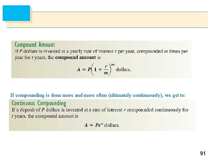
If compounding is done more and more often (ultimately continuously), we get to: 91

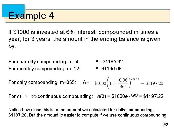
Example 4 If $1000 is invested at 6% interest, compounded m times a year, for 3 years, the amount in the ending balance is given by: For quarterly compounding, m=4: For monthly compounding, m=12: For daily compounding, m=365: For m A= $1195. 62 A=$1196. 68 A= continuous compounding: A(3) = $1000 e(0. 06)3 = $1197. 22 Notice how close this is to the amount we calculated for daily compounding, $1197. 20. But the amount is easier to compute if we use continuous compounding. 92

6. 6 Inverse Trigonometric Functions 93

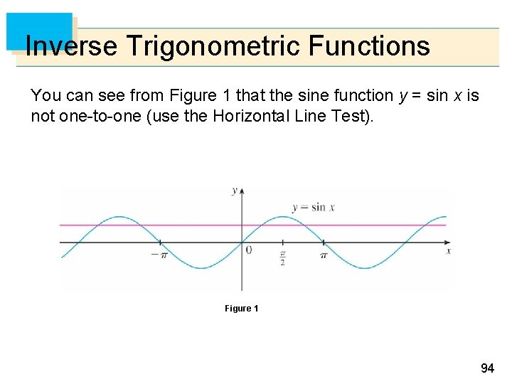
Inverse Trigonometric Functions You can see from Figure 1 that the sine function y = sin x is not one-to-one (use the Horizontal Line Test). Figure 1 94

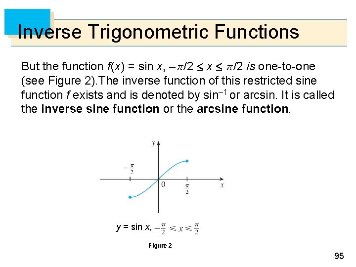
Inverse Trigonometric Functions But the function f (x) = sin x, – /2 x /2 is one-to-one (see Figure 2). The inverse function of this restricted sine function f exists and is denoted by sin– 1 or arcsin. It is called the inverse sine function or the arcsine function. y = sin x, Figure 2 95

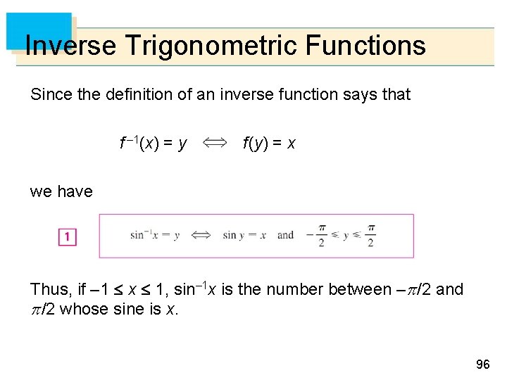
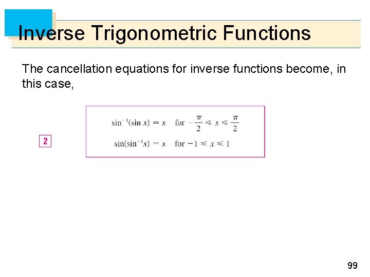
Inverse Trigonometric Functions Since the definition of an inverse function says that f – 1(x) = y f (y) = x we have Thus, if – 1 x 1, sin– 1 x is the number between – /2 and /2 whose sine is x. 96

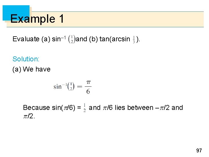
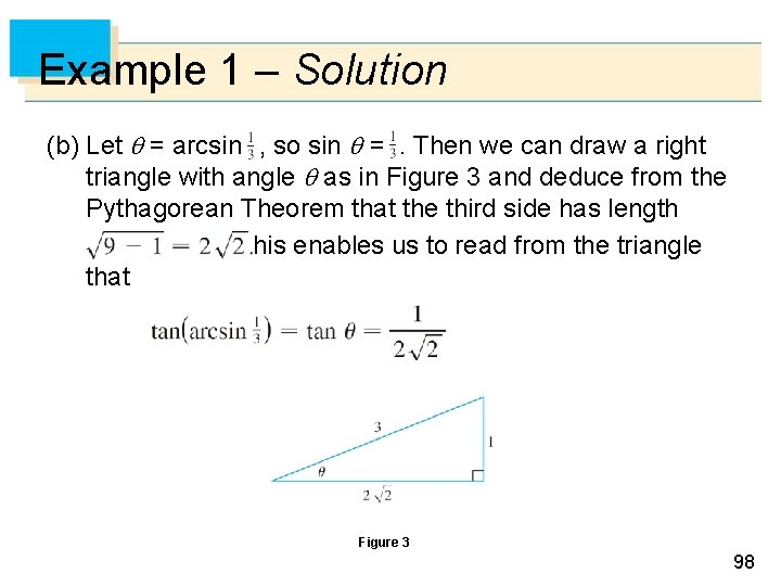
Example 1 Evaluate (a) sin– 1 and (b) tan(arcsin ). Solution: (a) We have Because sin( /6) = /2. and /6 lies between – /2 and 97

Example 1 – Solution (b) Let = arcsin , so sin =. Then we can draw a right triangle with angle as in Figure 3 and deduce from the Pythagorean Theorem that the third side has length This enables us to read from the triangle that Figure 3 98

Inverse Trigonometric Functions The cancellation equations for inverse functions become, in this case, 99

Inverse Trigonometric Functions The inverse sine function, sin– 1, has domain [– 1, 1] and range [– /2, /2], and its graph, shown in Figure 4, is obtained from that of the restricted sine function (Figure 2) by reflection about the line y = x. y = sin– 1 x = arcsin x Figure 4 100

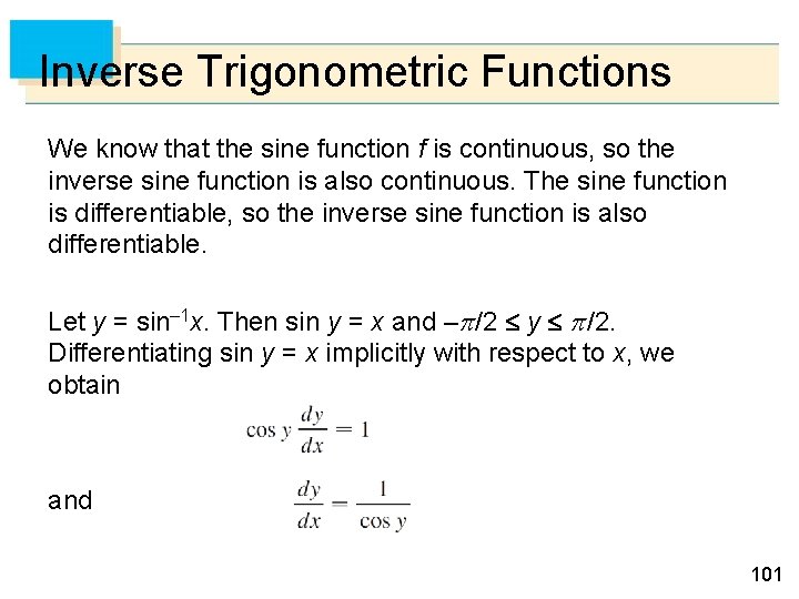
Inverse Trigonometric Functions We know that the sine function f is continuous, so the inverse sine function is also continuous. The sine function is differentiable, so the inverse sine function is also differentiable. Let y = sin– 1 x. Then sin y = x and – /2 y /2. Differentiating sin y = x implicitly with respect to x, we obtain and 101

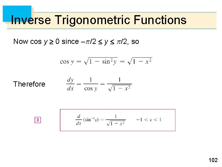
Inverse Trigonometric Functions Now cos y 0 since – /2 y /2, so Therefore 102

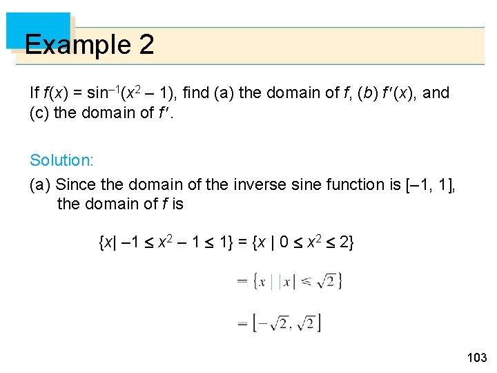
Example 2 If f (x) = sin– 1(x 2 – 1), find (a) the domain of f, (b) f (x), and (c) the domain of f . Solution: (a) Since the domain of the inverse sine function is [– 1, 1], the domain of f is {x| – 1 x 2 – 1 1} = {x | 0 x 2 2} 103

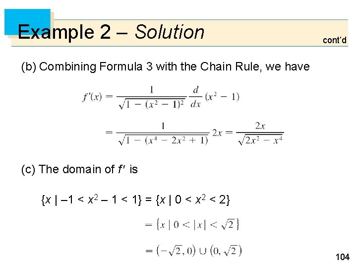
Example 2 – Solution cont’d (b) Combining Formula 3 with the Chain Rule, we have (c) The domain of f is {x | – 1 < x 2 – 1 < 1} = {x | 0 < x 2 < 2} 104

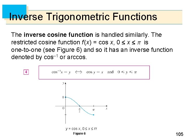
Inverse Trigonometric Functions The inverse cosine function is handled similarly. The restricted cosine function f (x) = cos x, 0 x is one-to-one (see Figure 6) and so it has an inverse function denoted by cos– 1 or arccos. y = cos x, 0 x π Figure 6 105

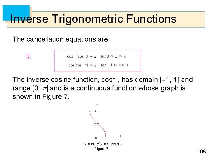
Inverse Trigonometric Functions The cancellation equations are The inverse cosine function, cos– 1, has domain [– 1, 1] and range [0, ] and is a continuous function whose graph is shown in Figure 7. y = cos– 1 x = arccos x Figure 7 106

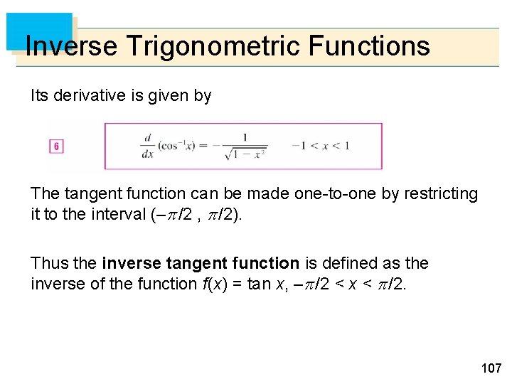
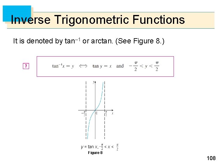
Inverse Trigonometric Functions Its derivative is given by The tangent function can be made one-to-one by restricting it to the interval (– /2 , /2). Thus the inverse tangent function is defined as the inverse of the function f (x) = tan x, – /2 < x < /2. 107

Inverse Trigonometric Functions It is denoted by tan– 1 or arctan. (See Figure 8. ) y = tan x, <x< Figure 8 108

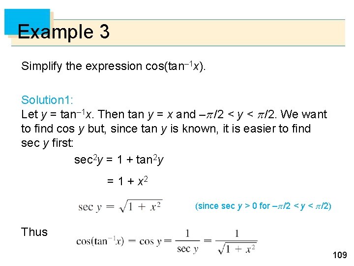
Example 3 Simplify the expression cos(tan– 1 x). Solution 1: Let y = tan– 1 x. Then tan y = x and – /2 < y < /2. We want to find cos y but, since tan y is known, it is easier to find sec y first: sec 2 y = 1 + tan 2 y = 1 + x 2 (since sec y > 0 for – /2 < y < /2) Thus 109

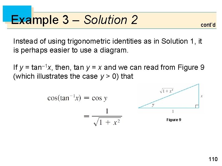
Example 3 – Solution 2 cont’d Instead of using trigonometric identities as in Solution 1, it is perhaps easier to use a diagram. If y = tan– 1 x, then, tan y = x and we can read from Figure 9 (which illustrates the case y > 0) that Figure 9 110

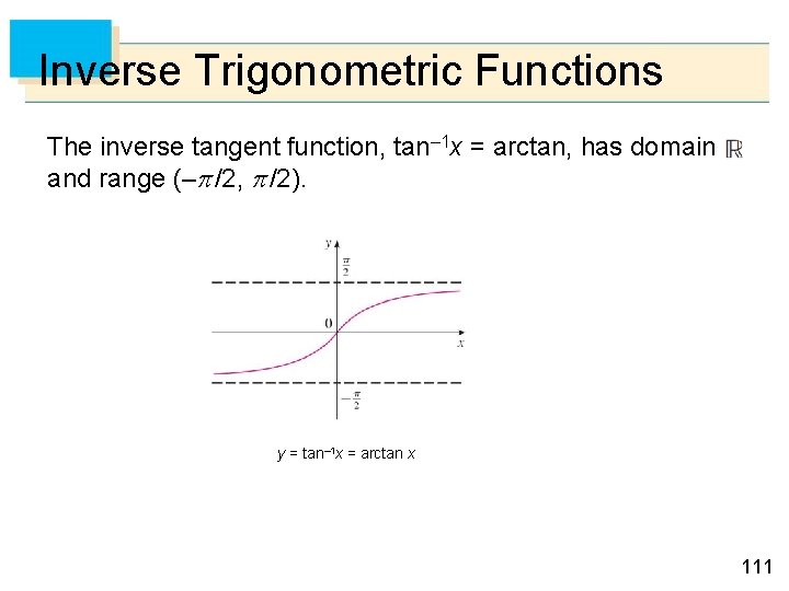
Inverse Trigonometric Functions The inverse tangent function, tan– 1 x = arctan, has domain and range (– /2, /2). y = tan– 1 x = arctan x 111

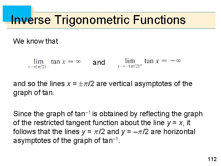
Inverse Trigonometric Functions We know that and so the lines x = /2 are vertical asymptotes of the graph of tan. Since the graph of tan– 1 is obtained by reflecting the graph of the restricted tangent function about the line y = x, it follows that the lines y = /2 and y = – /2 are horizontal asymptotes of the graph of tan– 1. 112

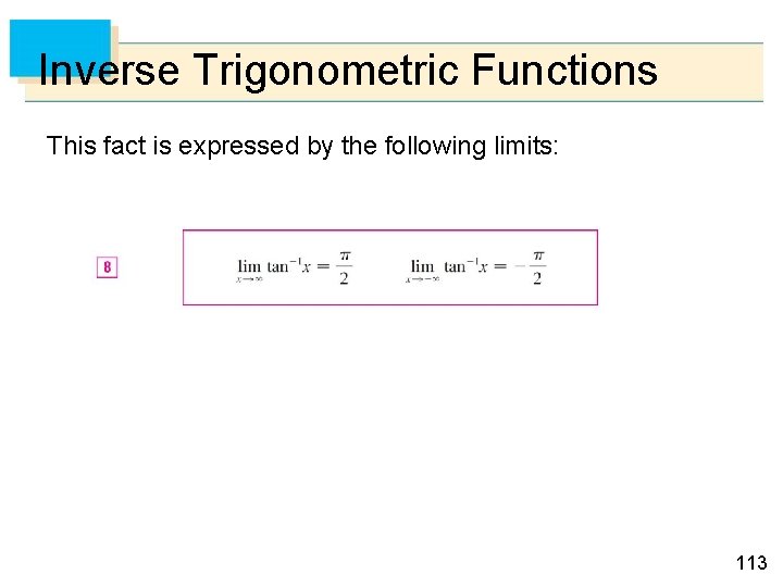
Inverse Trigonometric Functions This fact is expressed by the following limits: 113

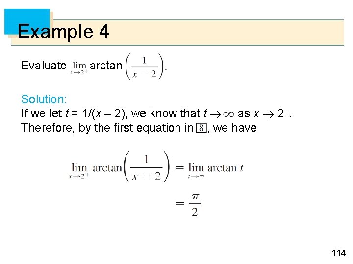
Example 4 Evaluate arctan Solution: If we let t = 1/(x – 2), we know that t as x 2+. Therefore, by the first equation in , we have 114

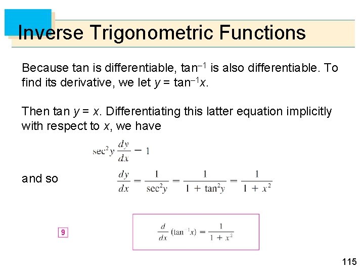
Inverse Trigonometric Functions Because tan is differentiable, tan– 1 is also differentiable. To find its derivative, we let y = tan– 1 x. Then tan y = x. Differentiating this latter equation implicitly with respect to x, we have and so 115

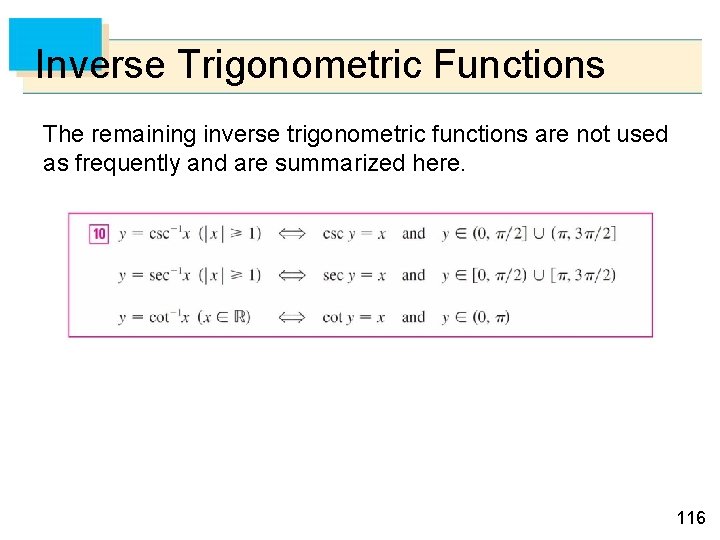
Inverse Trigonometric Functions The remaining inverse trigonometric functions are not used as frequently and are summarized here. 116

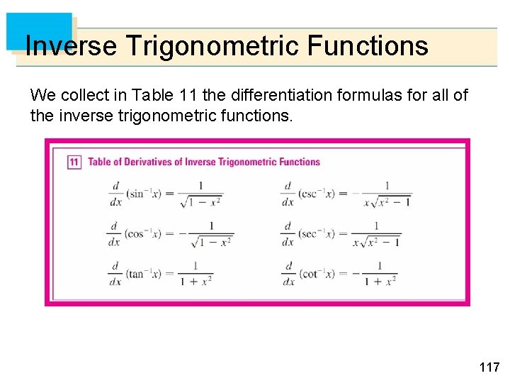
Inverse Trigonometric Functions We collect in Table 11 the differentiation formulas for all of the inverse trigonometric functions. 117

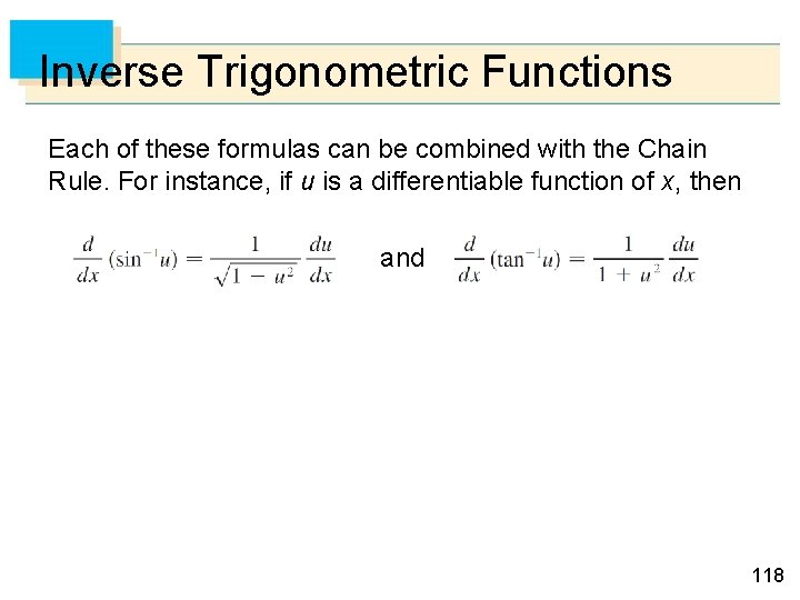
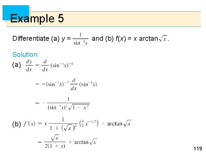
Inverse Trigonometric Functions Each of these formulas can be combined with the Chain Rule. For instance, if u is a differentiable function of x, then and 118

Example 5 Differentiate (a) y = and (b) f (x) = x arctan . Solution: (a) (b) 119

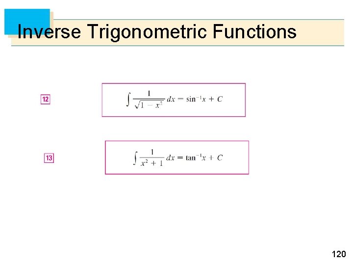
Inverse Trigonometric Functions 120

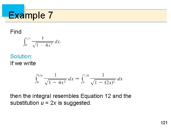
Example 7 Find Solution: If we write then the integral resembles Equation 12 and the substitution u = 2 x is suggested. 121

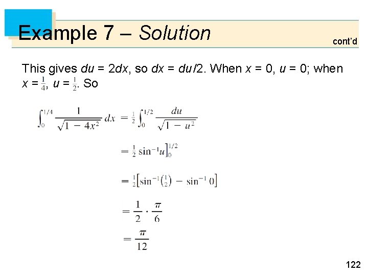
Example 7 – Solution cont’d This gives du = 2 dx, so dx = du /2. When x = 0, u = 0; when x = , u =. So 122

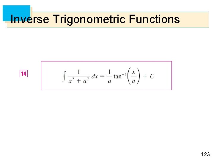
Inverse Trigonometric Functions 123

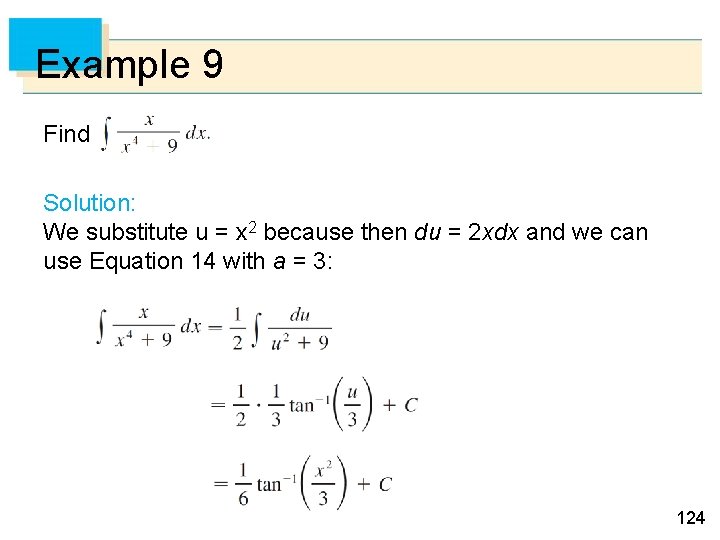
Example 9 Find Solution: We substitute u = x 2 because then du = 2 xdx and we can use Equation 14 with a = 3: 124

6. 8 Indeterminate Forms and l’Hospital’s Rule 125

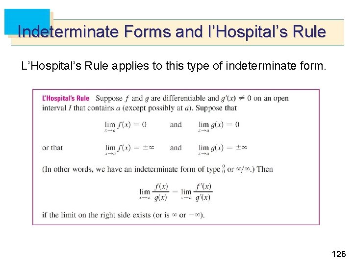
Indeterminate Forms and l’Hospital’s Rule L’Hospital’s Rule applies to this type of indeterminate form. 126

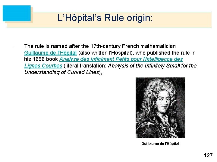
L’Hôpital’s Rule origin: . The rule is named after the 17 th-century French mathematician Guillaume de l'Hôpital (also written l'Hospital), who published the rule in his 1696 book Analyse des Infiniment Petits pour l'Intelligence des Lignes Courbes (literal translation: Analysis of the Infinitely Small for the Understanding of Curved Lines), Guillaume de l'Hôpital 127

Indeterminate Forms and l’Hospital’s Rule Note 1: L’Hospital’s Rule says that the limit of a quotient of functions is equal to the limit of the quotient of their derivatives, provided that the given conditions are satisfied. It is especially important to verify the conditions regarding the limits of f and g before using l’Hospital’s Rule. Note 2: L’Hospital’s Rule is also valid for one-sided limits and for limits at infinity or negative infinity; that is, “x a” can be replaced by any of the symbols x a+, x a–, x , or x –. 128

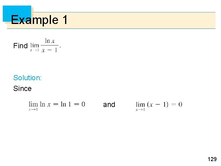
Example 1 Find Solution: Since and 129

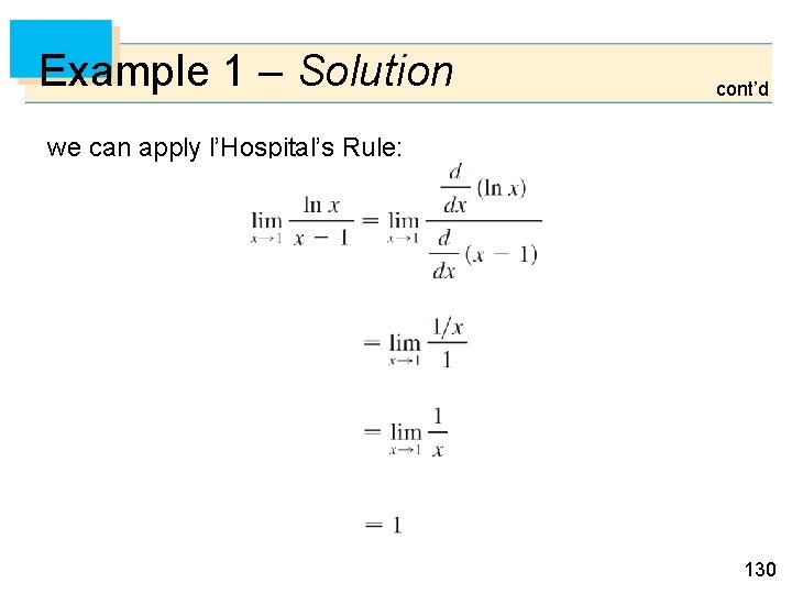
Example 1 – Solution cont’d we can apply l’Hospital’s Rule: 130

Indeterminate Products 131

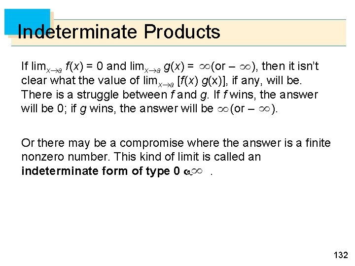
Indeterminate Products If limx a f (x) = 0 and limx a g(x) = (or – ), then it isn’t clear what the value of limx a [f (x) g(x)], if any, will be. There is a struggle between f and g. If f wins, the answer will be 0; if g wins, the answer will be (or – ). Or there may be a compromise where the answer is a finite nonzero number. This kind of limit is called an indeterminate form of type 0 . 132

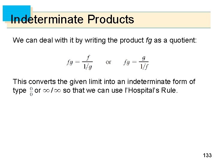
Indeterminate Products We can deal with it by writing the product fg as a quotient: This converts the given limit into an indeterminate form of type or / so that we can use l’Hospital’s Rule. 133

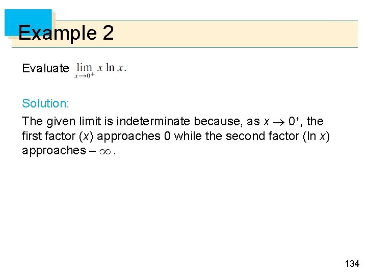
Example 2 Evaluate Solution: The given limit is indeterminate because, as x 0+, the first factor (x) approaches 0 while the second factor (ln x) approaches –. 134

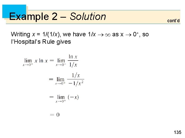
Example 2 – Solution Writing x = 1/(1/x), we have 1/x l’Hospital’s Rule gives cont’d as x 0+, so 135

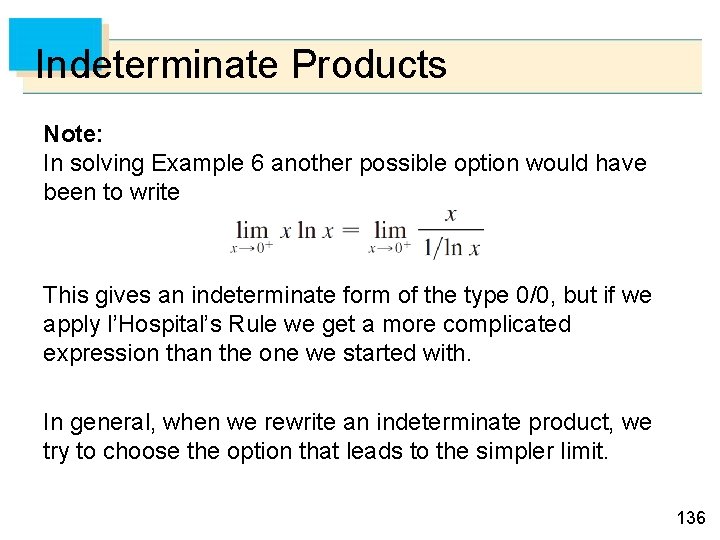
Indeterminate Products Note: In solving Example 6 another possible option would have been to write This gives an indeterminate form of the type 0/0, but if we apply l’Hospital’s Rule we get a more complicated expression than the one we started with. In general, when we rewrite an indeterminate product, we try to choose the option that leads to the simpler limit. 136

Indeterminate Differences 137

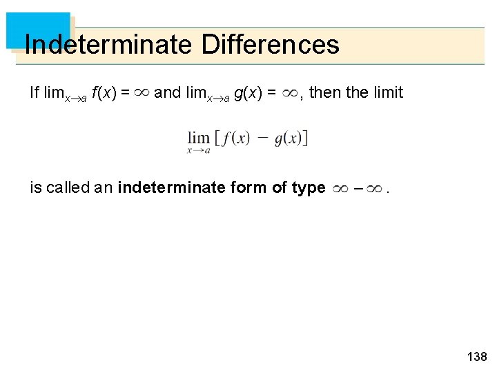
Indeterminate Differences If limx a f (x) = and limx a g(x) = , then the limit is called an indeterminate form of type – . 138

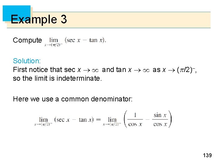
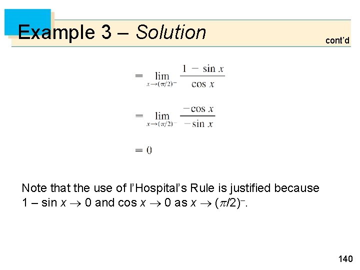
Example 3 Compute Solution: First notice that sec x and tan x so the limit is indeterminate. as x ( /2)–, Here we use a common denominator: 139

Example 3 – Solution cont’d Note that the use of l’Hospital’s Rule is justified because 1 – sin x 0 and cos x 0 as x ( /2)–. 140

Indeterminate Powers 141

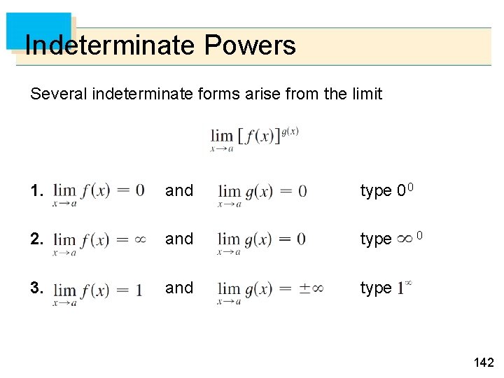
Indeterminate Powers Several indeterminate forms arise from the limit 1. and type 0 0 2. and type 3. and type 0 142

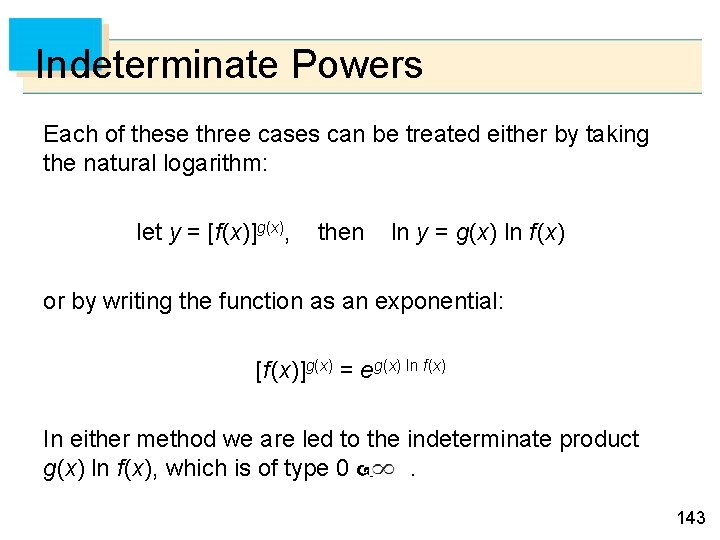
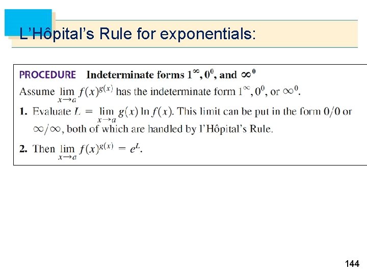
Indeterminate Powers Each of these three cases can be treated either by taking the natural logarithm: let y = [f (x)]g(x), then ln y = g(x) ln f (x) or by writing the function as an exponential: [f (x)]g(x) = eg (x) ln f (x) In either method we are led to the indeterminate product g(x) ln f (x), which is of type 0 . 143

L’Hôpital’s Rule for exponentials: 144

Practice problems: Visit the following sites to practice more: • http: //tutorial. math. lamar. edu/problems/calci/lhospitalsrule. aspx • http: //www. millersville. edu/~bikenaga/calculus/lhopit. html 145

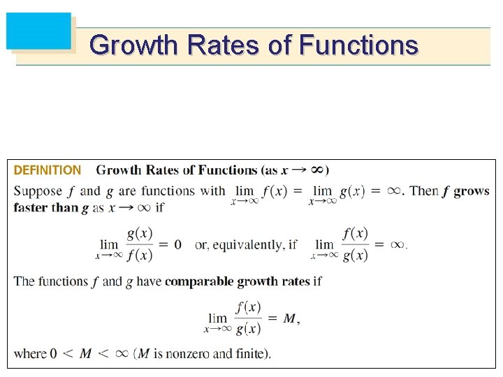
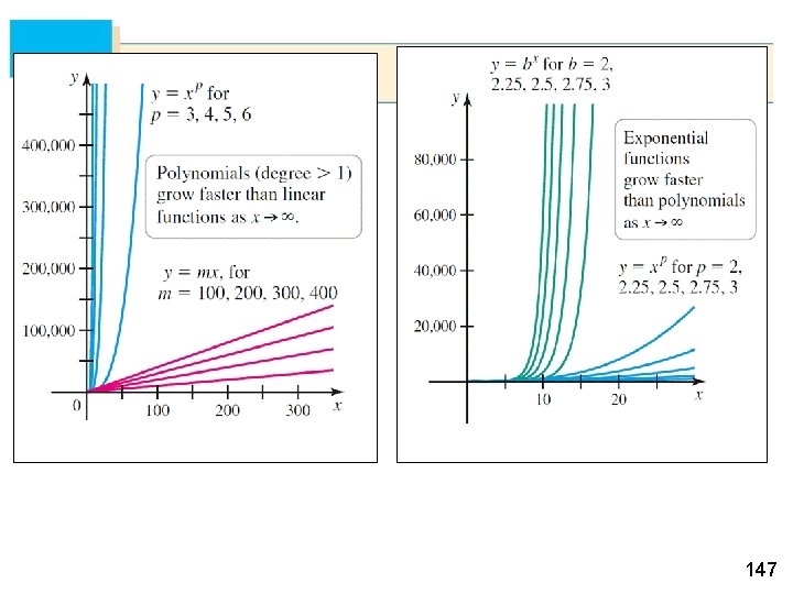
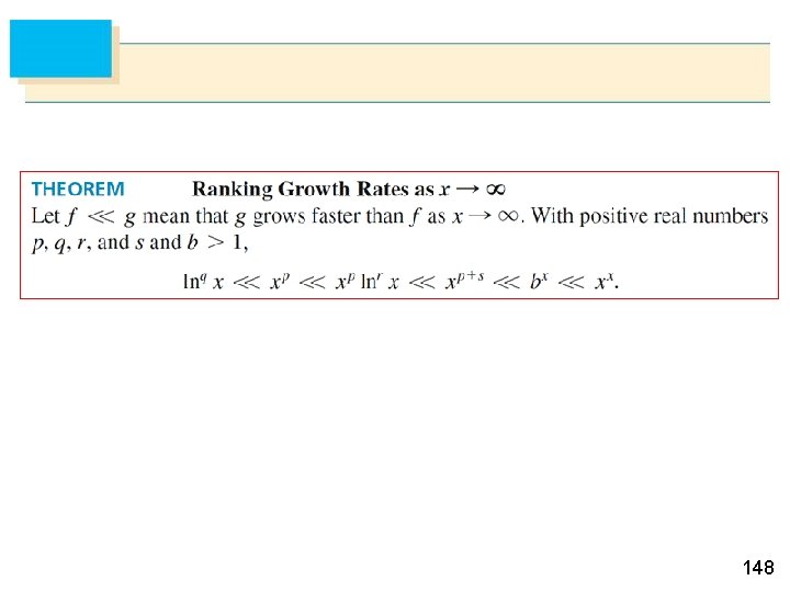
Growth Rates of Functions 146

147

148