Inverse Laplace Transform 1 Contour Integration Mathematical Topic

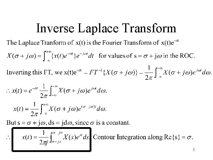
Inverse Laplace Transform 1

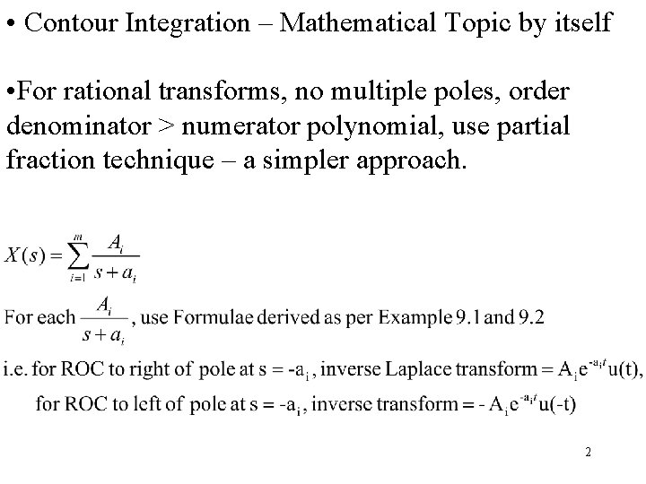
• Contour Integration – Mathematical Topic by itself • For rational transforms, no multiple poles, order denominator > numerator polynomial, use partial fraction technique – a simpler approach. 2

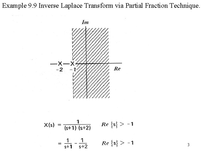
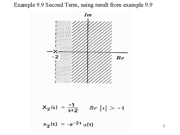
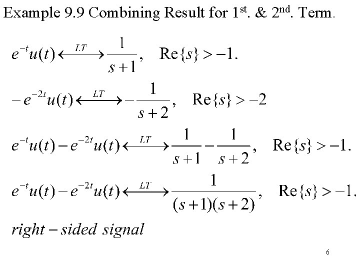
Example 9. 9 Inverse Laplace Transform via Partial Fraction Technique. 3

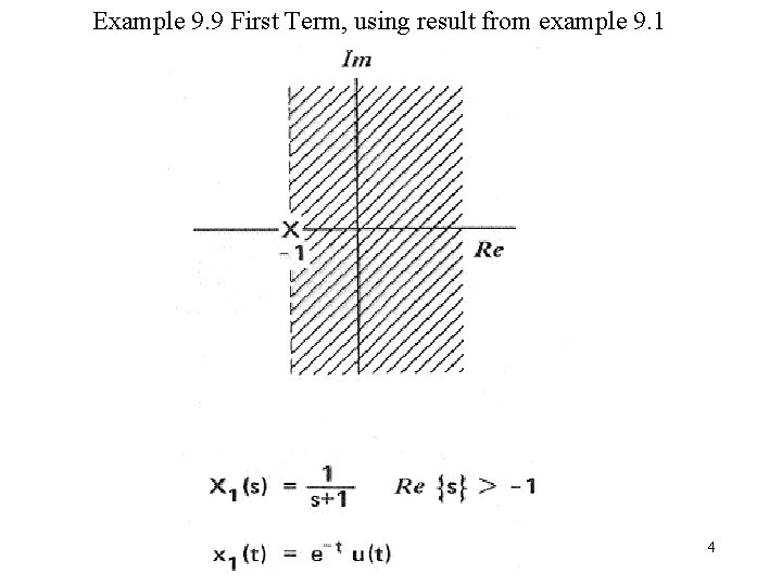
Example 9. 9 First Term, using result from example 9. 1 4

Example 9. 9 Second Term, using result from example 9. 9 5

Example 9. 9 Combining Result for 1 st. & 2 nd. Term. 6

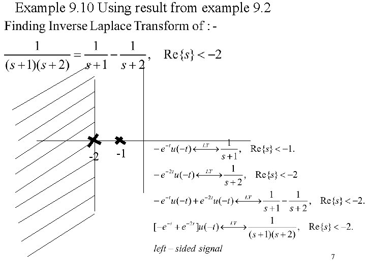
Example 9. 10 Using result from example 9. 2 -2 -1 7

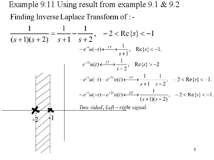
Example 9. 11 Using result from example 9. 1 & 9. 2 -2 -1 8

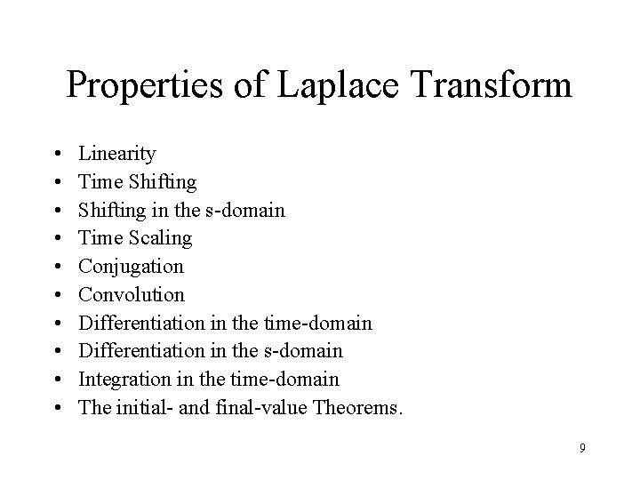
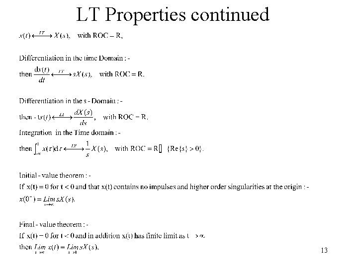
Properties of Laplace Transform • • • Linearity Time Shifting in the s-domain Time Scaling Conjugation Convolution Differentiation in the time-domain Differentiation in the s-domain Integration in the time-domain The initial- and final-value Theorems. 9

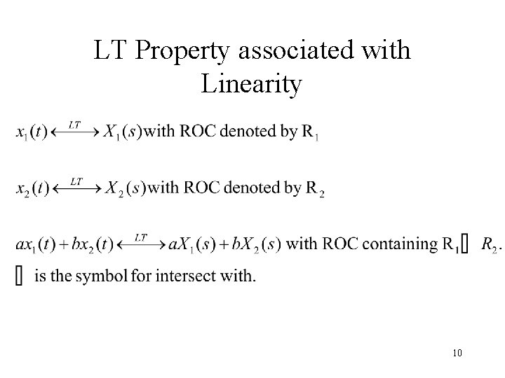
LT Property associated with Linearity 10

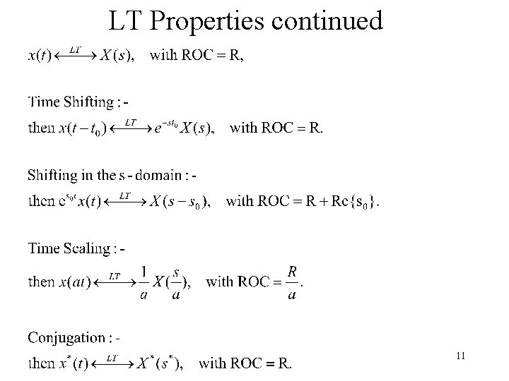
LT Properties continued 11

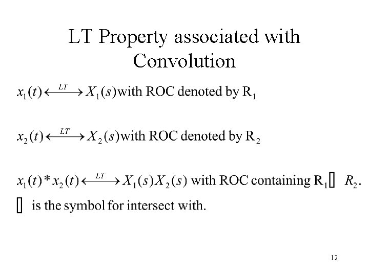
LT Property associated with Convolution 12

LT Properties continued 13

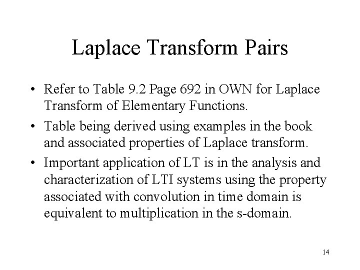
Laplace Transform Pairs • Refer to Table 9. 2 Page 692 in OWN for Laplace Transform of Elementary Functions. • Table being derived using examples in the book and associated properties of Laplace transform. • Important application of LT is in the analysis and characterization of LTI systems using the property associated with convolution in time domain is equivalent to multiplication in the s-domain. 14

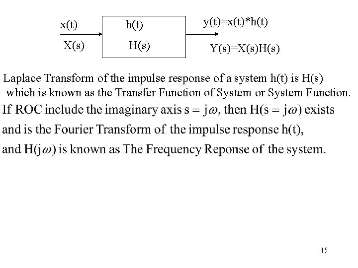
x(t) h(t) X(s) H(s) y(t)=x(t)*h(t) Y(s)=X(s)H(s) Laplace Transform of the impulse response of a system h(t) is H(s) which is known as the Transfer Function of System or System Function. 15

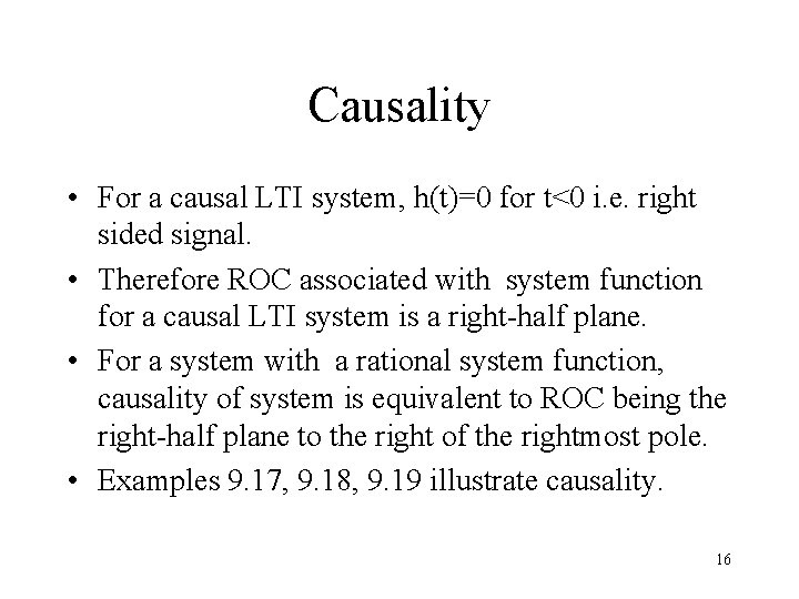
Causality • For a causal LTI system, h(t)=0 for t<0 i. e. right sided signal. • Therefore ROC associated with system function for a causal LTI system is a right-half plane. • For a system with a rational system function, causality of system is equivalent to ROC being the right-half plane to the right of the rightmost pole. • Examples 9. 17, 9. 18, 9. 19 illustrate causality. 16

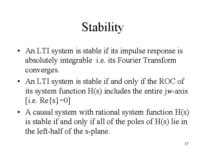
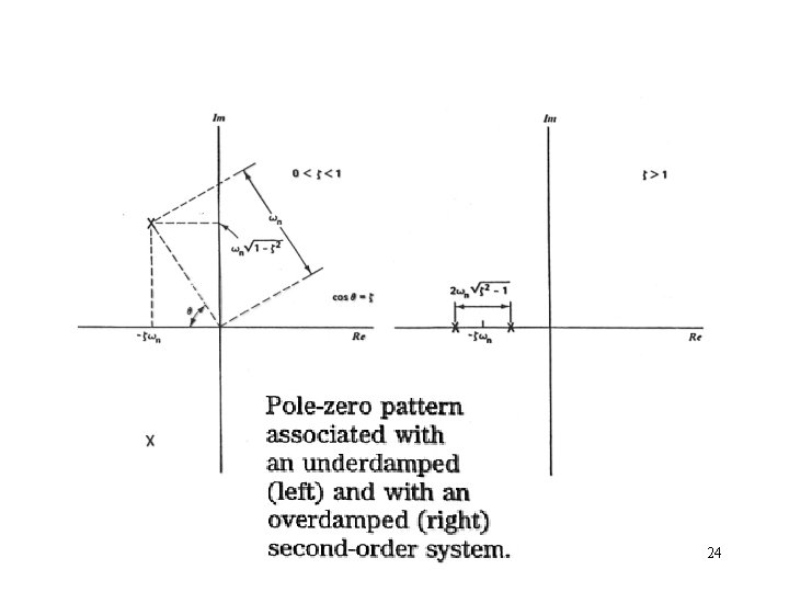
Stability • An LTI system is stable if its impulse response is absolutely integrable i. e. its Fourier Transform converges. • An LTI system is stable if and only if the ROC of its system function H(s) includes the entire jw-axis [i. e. Re{s}=0] • A causal system with rational system function H(s) is stable if and only if all of the poles of H(s) lie in the left-half of the s-plane. 17

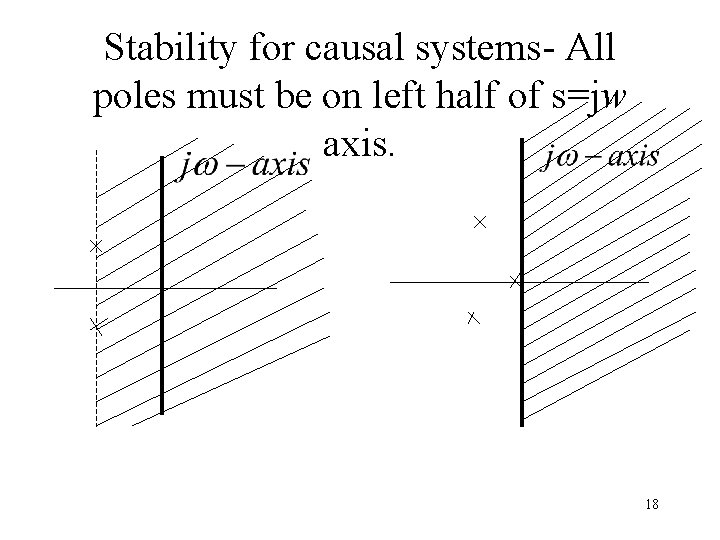
Stability for causal systems- All poles must be on left half of s=jw axis. 18

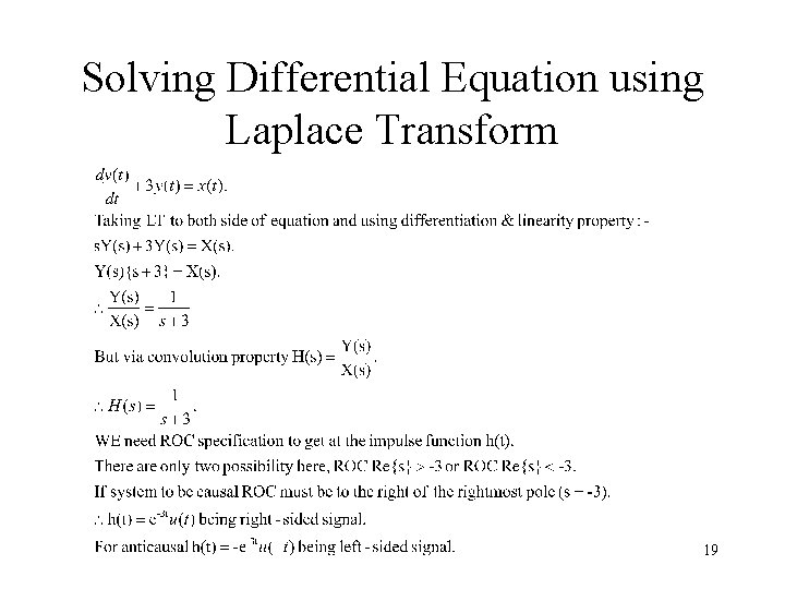
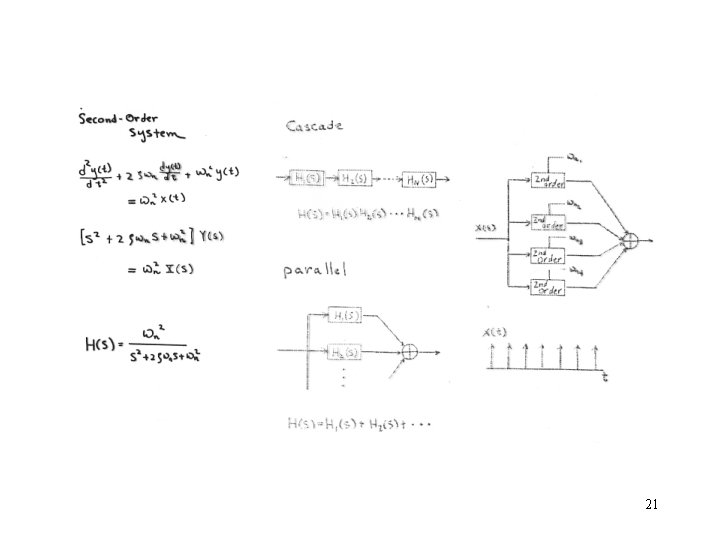
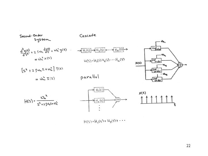
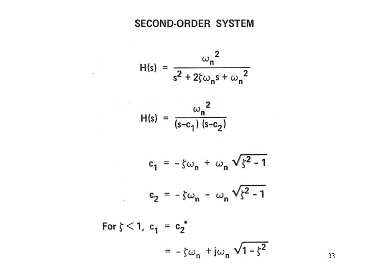
Solving Differential Equation using Laplace Transform 19

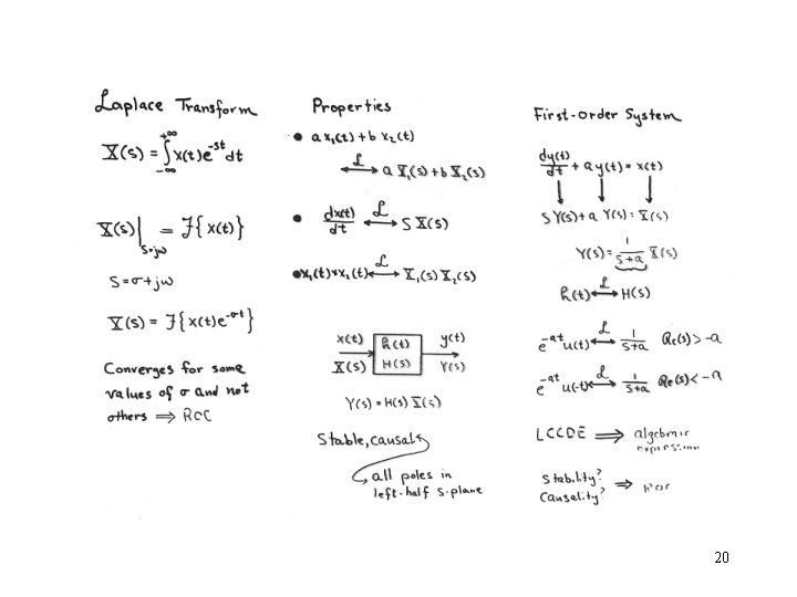
20

21

22

23

24

25

26

27