Chapter 13 Generalized Linear Models Linear Regression Analysis

Chapter 13 Generalized Linear Models Linear Regression Analysis 5 E Montgomery, Peck & Vining 1

Generalized Linear Models • Traditional applications of linear models, such as DOX and multiple linear regression, assume that the response variable is – Normally distributed – Constant variance – Independent • There are many situations where these assumptions are inappropriate – The response is either binary (0, 1), or a count – The response is continuous, but nonnormal Linear Regression Analysis 5 E Montgomery, Peck & Vining 2

Some Approaches to These Problems • Data transformation – Induce approximate normality – Stabilize variance – Simplify model form • Weighted least squares – Often used to stabilize variance • Generalized linear models (GLM) – Approach is about 25 -30 years old, unifies linear and nonlinear regression models – Response distribution is a member of the exponential family (normal, exponential, gamma, binomial, Poisson) Linear Regression Analysis 5 E Montgomery, Peck & Vining 3

Generalized Linear Models • Original applications were in biopharmaceutical sciences • Lots of recent interest in GLMs in industrial statistics • GLMs are simple models; include linear regression and OLS as a special case • Parameter estimation is by maximum likelihood (assume that the response distribution is known) • Inference on parameters is based on large-sample or asymptotic theory • We will consider logistic regression, Poisson regression, then the GLM Linear Regression Analysis 5 E Montgomery, Peck & Vining 4

References • Montgomery, D. C. , Peck, E. A 5, and Vining, G. G. (2012), Introduction to Linear Regression Analysis, 4 th Edition, Wiley, New York (see Chapter 14) • Myers, R. H. , Montgomery, D. C. , Vining, G. G. and Robinson, T. J. (2010), Generalized Linear Models with Applications in Engineering and the Sciences, 2 nd edition, Wiley, New York • Hosmer, D. W. and Lemeshow, S. (2000), Applied Logistic Regression, 2 nd Edition, Wiley, New York • Lewis, S. L. , Montgomery, D. C. , and Myers, R. H. (2001), “Confidence Interval Coverage for Designed Experiments Analyzed with GLMs”, Journal of Quality Technology 33, pp. 279 -292 • Lewis, S. L. , Montgomery, D. C. , and Myers, R. H. (2001), “Examples of Designed Experiments with Nonnormal Responses”, Journal of Quality Technology 33, pp. 265 -278 • Myers, R. H. and Montgomery, D. C. (1997), “A Tutorial on Generalized Linear Models”, Journal of Quality Technology 29, pp. 274 -291 Linear Regression Analysis 5 E Montgomery, Peck & Vining 5

Binary Response Variables • The outcome ( or response, or endpoint) values 0, 1 can represent “success” and “failure” • Occurs often in the biopharmaceutical field; doseresponse studies, bioassays, clinical trials • Industrial applications include failure analysis, fatigue testing, reliability testing • For example, functional electrical testing on a semiconductor can yield: – “success” in which case the device works – “failure” due to a short, an open, or some other failure mode Linear Regression Analysis 5 E Montgomery, Peck & Vining 6

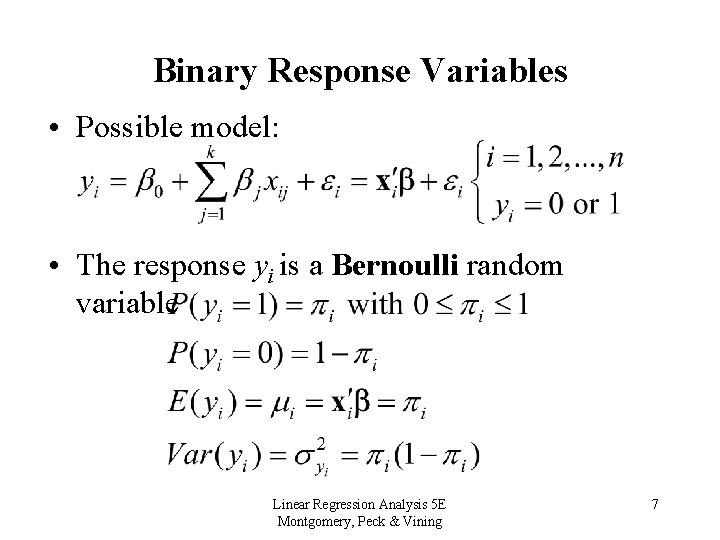
Binary Response Variables • Possible model: • The response yi is a Bernoulli random variable Linear Regression Analysis 5 E Montgomery, Peck & Vining 7

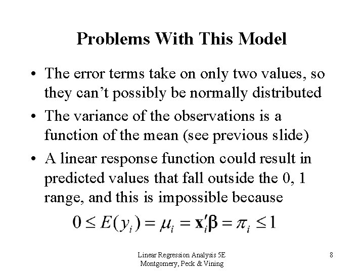
Problems With This Model • The error terms take on only two values, so they can’t possibly be normally distributed • The variance of the observations is a function of the mean (see previous slide) • A linear response function could result in predicted values that fall outside the 0, 1 range, and this is impossible because Linear Regression Analysis 5 E Montgomery, Peck & Vining 8

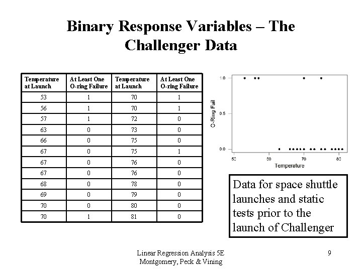
Binary Response Variables – The Challenger Data Temperature at Launch At Least One O-ring Failure 53 1 70 1 56 1 70 1 57 1 72 0 63 0 73 0 66 0 75 0 67 0 75 1 67 0 76 0 68 0 78 0 69 0 70 0 80 0 70 1 81 0 Linear Regression Analysis 5 E Montgomery, Peck & Vining Data for space shuttle launches and static tests prior to the launch of Challenger 9

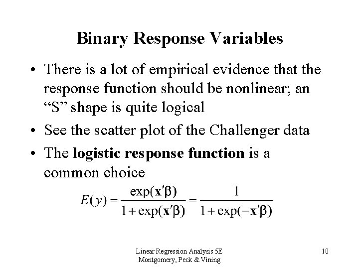
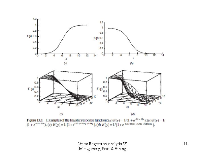
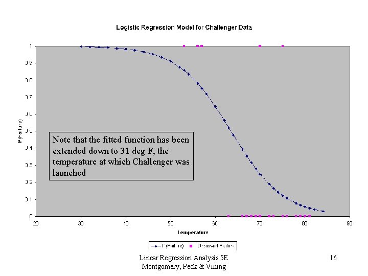
Binary Response Variables • There is a lot of empirical evidence that the response function should be nonlinear; an “S” shape is quite logical • See the scatter plot of the Challenger data • The logistic response function is a common choice Linear Regression Analysis 5 E Montgomery, Peck & Vining 10

Linear Regression Analysis 5 E Montgomery, Peck & Vining 11

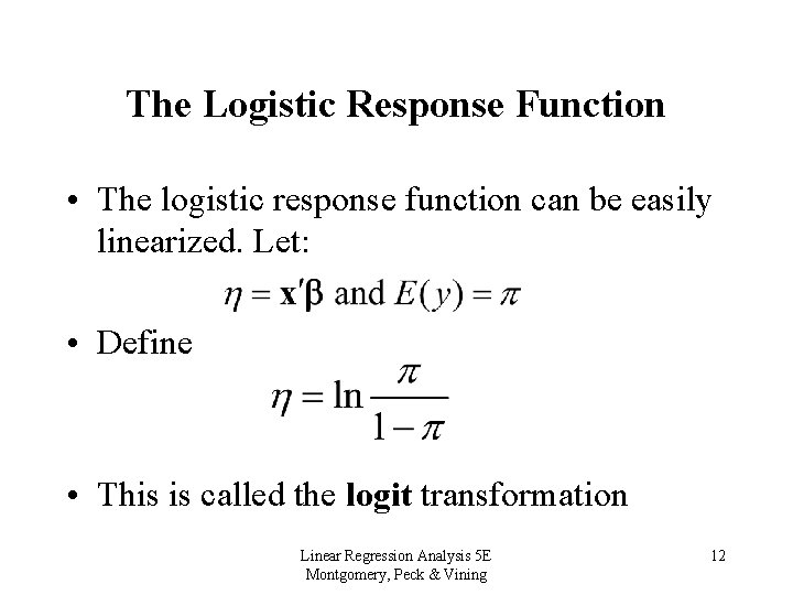
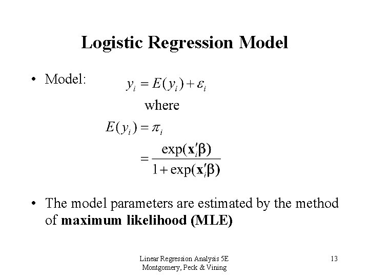
The Logistic Response Function • The logistic response function can be easily linearized. Let: • Define • This is called the logit transformation Linear Regression Analysis 5 E Montgomery, Peck & Vining 12

Logistic Regression Model • Model: • The model parameters are estimated by the method of maximum likelihood (MLE) Linear Regression Analysis 5 E Montgomery, Peck & Vining 13

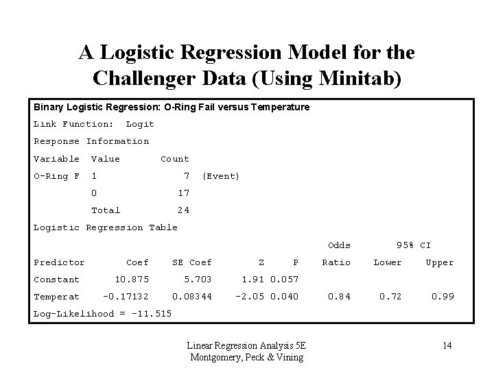
A Logistic Regression Model for the Challenger Data (Using Minitab) Binary Logistic Regression: O-Ring Fail versus Temperature Link Function: Logit Response Information Variable Value Count O-Ring F 1 7 0 17 Total 24 (Event) Logistic Regression Table Odds Predictor Coef SE Coef Z P Constant 10. 875 5. 703 1. 91 0. 057 Temperat -0. 17132 0. 08344 -2. 05 0. 040 95% CI Ratio Lower Upper 0. 84 0. 72 0. 99 Log-Likelihood = -11. 515 Linear Regression Analysis 5 E Montgomery, Peck & Vining 14

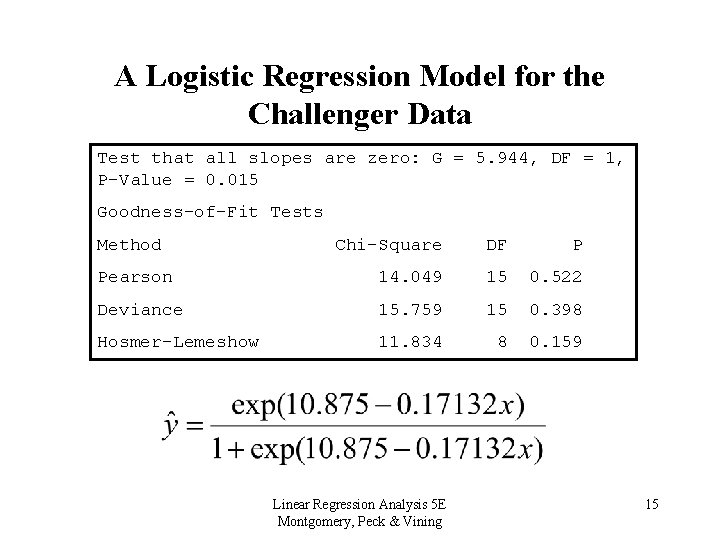
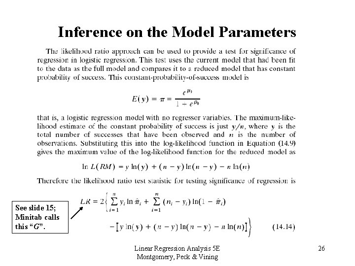
A Logistic Regression Model for the Challenger Data Test that all slopes are zero: G = 5. 944, DF = 1, P-Value = 0. 015 Goodness-of-Fit Tests Method Chi-Square DF P Pearson 14. 049 15 0. 522 Deviance 15. 759 15 0. 398 Hosmer-Lemeshow 11. 834 8 0. 159 Linear Regression Analysis 5 E Montgomery, Peck & Vining 15

Note that the fitted function has been extended down to 31 deg F, the temperature at which Challenger was launched Linear Regression Analysis 5 E Montgomery, Peck & Vining 16

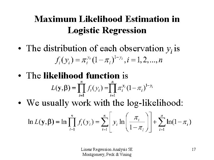
Maximum Likelihood Estimation in Logistic Regression • The distribution of each observation yi is • The likelihood function is • We usually work with the log-likelihood: Linear Regression Analysis 5 E Montgomery, Peck & Vining 17

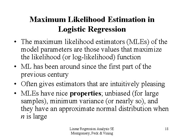
Maximum Likelihood Estimation in Logistic Regression • The maximum likelihood estimators (MLEs) of the model parameters are those values that maximize the likelihood (or log-likelihood) function • ML has been around since the first part of the previous century • Often gives estimators that are intuitively pleasing • MLEs have nice properties; unbiased (for large samples), minimum variance (or nearly so), and they have an approximate normal distribution when n is large Linear Regression Analysis 5 E Montgomery, Peck & Vining 18

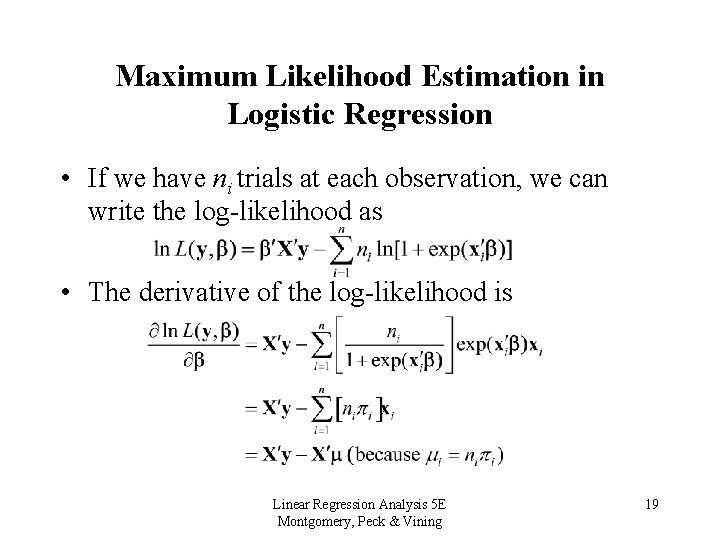
Maximum Likelihood Estimation in Logistic Regression • If we have ni trials at each observation, we can write the log-likelihood as • The derivative of the log-likelihood is Linear Regression Analysis 5 E Montgomery, Peck & Vining 19

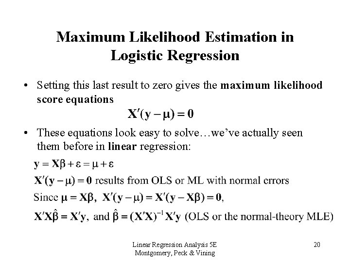
Maximum Likelihood Estimation in Logistic Regression • Setting this last result to zero gives the maximum likelihood score equations • These equations look easy to solve…we’ve actually seen them before in linear regression: Linear Regression Analysis 5 E Montgomery, Peck & Vining 20

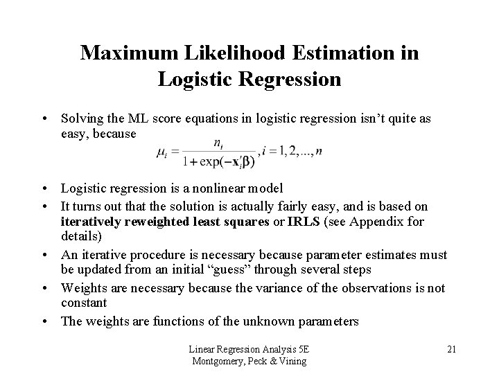
Maximum Likelihood Estimation in Logistic Regression • Solving the ML score equations in logistic regression isn’t quite as easy, because • Logistic regression is a nonlinear model • It turns out that the solution is actually fairly easy, and is based on iteratively reweighted least squares or IRLS (see Appendix for details) • An iterative procedure is necessary because parameter estimates must be updated from an initial “guess” through several steps • Weights are necessary because the variance of the observations is not constant • The weights are functions of the unknown parameters Linear Regression Analysis 5 E Montgomery, Peck & Vining 21

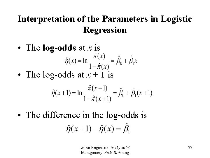
Interpretation of the Parameters in Logistic Regression • The log-odds at x is • The log-odds at x + 1 is • The difference in the log-odds is Linear Regression Analysis 5 E Montgomery, Peck & Vining 22

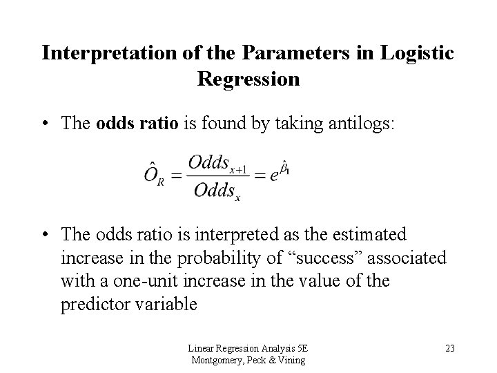
Interpretation of the Parameters in Logistic Regression • The odds ratio is found by taking antilogs: • The odds ratio is interpreted as the estimated increase in the probability of “success” associated with a one-unit increase in the value of the predictor variable Linear Regression Analysis 5 E Montgomery, Peck & Vining 23

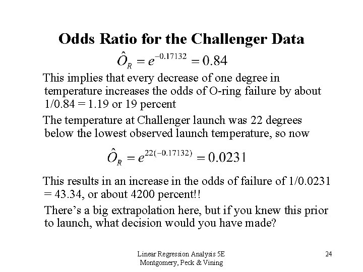
Odds Ratio for the Challenger Data This implies that every decrease of one degree in temperature increases the odds of O-ring failure by about 1/0. 84 = 1. 19 or 19 percent The temperature at Challenger launch was 22 degrees below the lowest observed launch temperature, so now This results in an increase in the odds of failure of 1/0. 0231 = 43. 34, or about 4200 percent!! There’s a big extrapolation here, but if you knew this prior to launch, what decision would you have made? Linear Regression Analysis 5 E Montgomery, Peck & Vining 24

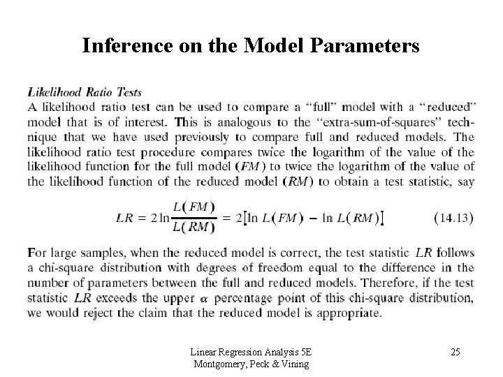
Inference on the Model Parameters Linear Regression Analysis 5 E Montgomery, Peck & Vining 25

Inference on the Model Parameters See slide 15; Minitab calls this “G”. Linear Regression Analysis 5 E Montgomery, Peck & Vining 26

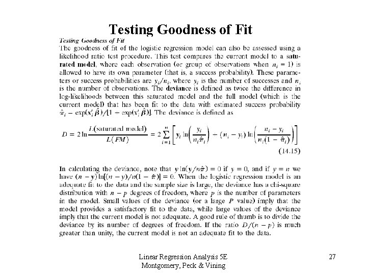
Testing Goodness of Fit Linear Regression Analysis 5 E Montgomery, Peck & Vining 27

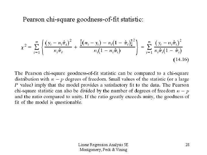
Pearson chi-square goodness-of-fit statistic: Linear Regression Analysis 5 E Montgomery, Peck & Vining 28

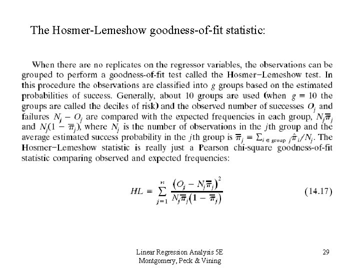
The Hosmer-Lemeshow goodness-of-fit statistic: Linear Regression Analysis 5 E Montgomery, Peck & Vining 29

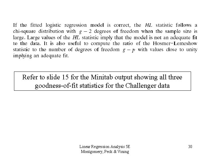
Refer to slide 15 for the Minitab output showing all three goodness-of-fit statistics for the Challenger data Linear Regression Analysis 5 E Montgomery, Peck & Vining 30

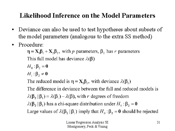
Likelihood Inference on the Model Parameters • Deviance can also be used to test hypotheses about subsets of the model parameters (analogous to the extra SS method) • Procedure: Linear Regression Analysis 5 E Montgomery, Peck & Vining 31

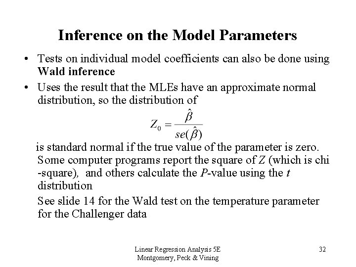
Inference on the Model Parameters • Tests on individual model coefficients can also be done using Wald inference • Uses the result that the MLEs have an approximate normal distribution, so the distribution of is standard normal if the true value of the parameter is zero. Some computer programs report the square of Z (which is chi -square), and others calculate the P-value using the t distribution See slide 14 for the Wald test on the temperature parameter for the Challenger data Linear Regression Analysis 5 E Montgomery, Peck & Vining 32

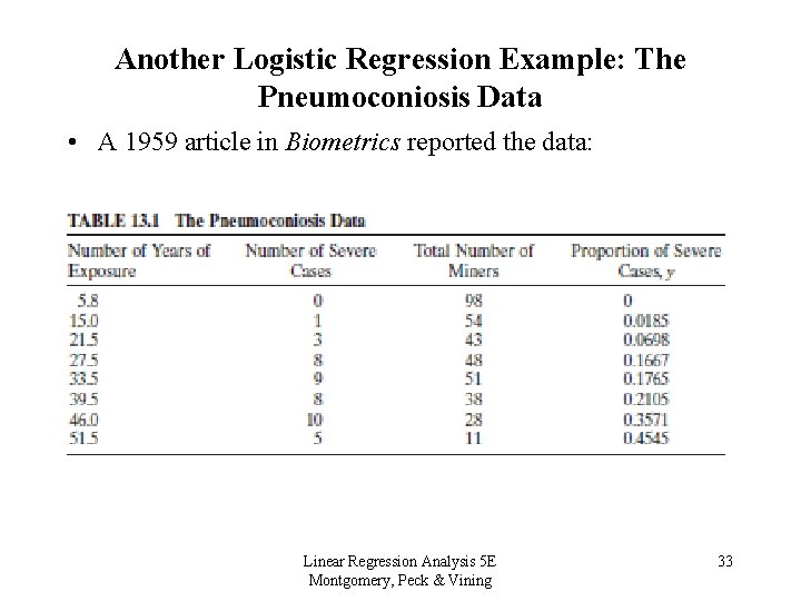
Another Logistic Regression Example: The Pneumoconiosis Data • A 1959 article in Biometrics reported the data: Linear Regression Analysis 5 E Montgomery, Peck & Vining 33

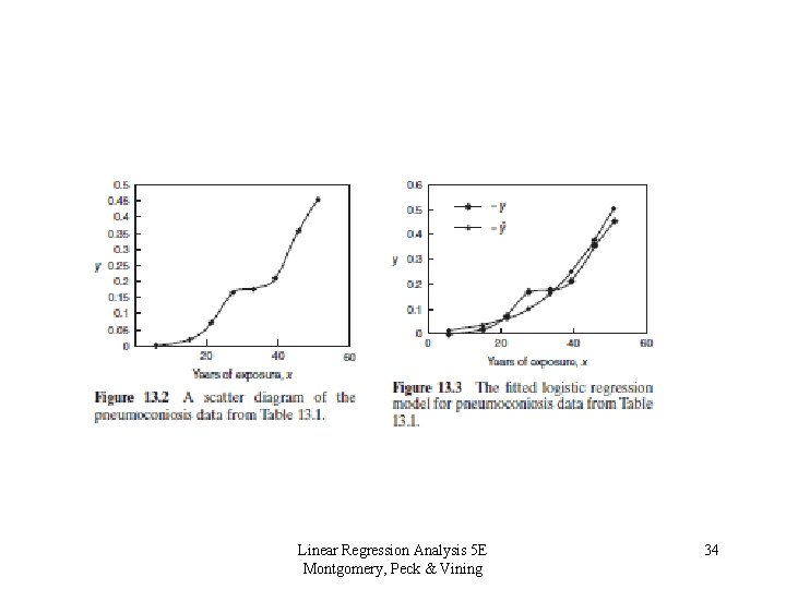
Linear Regression Analysis 5 E Montgomery, Peck & Vining 34

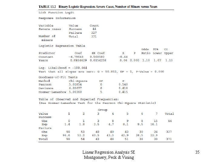
Linear Regression Analysis 5 E Montgomery, Peck & Vining 35

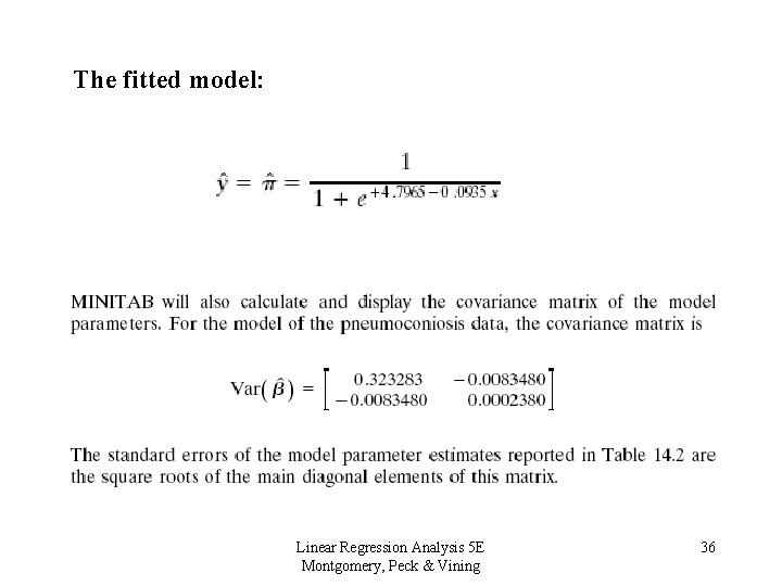
The fitted model: Linear Regression Analysis 5 E Montgomery, Peck & Vining 36

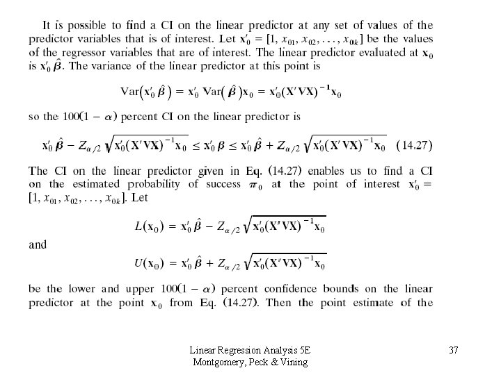
Linear Regression Analysis 5 E Montgomery, Peck & Vining 37

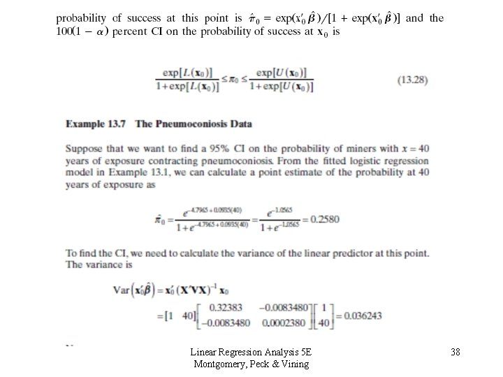
Linear Regression Analysis 5 E Montgomery, Peck & Vining 38

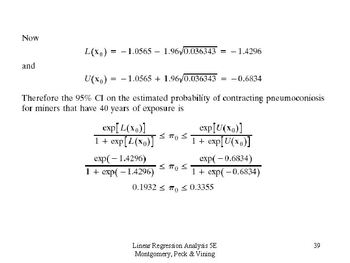
Linear Regression Analysis 5 E Montgomery, Peck & Vining 39

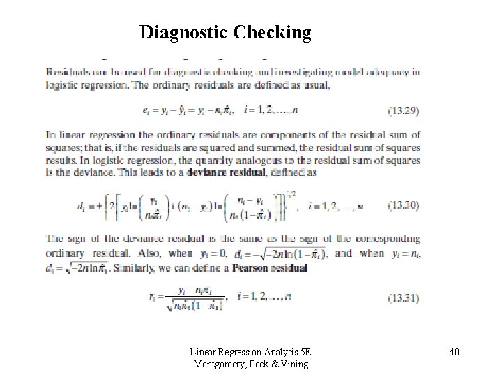
Diagnostic Checking Linear Regression Analysis 5 E Montgomery, Peck & Vining 40

Linear Regression Analysis 5 E Montgomery, Peck & Vining 41

Linear Regression Analysis 5 E Montgomery, Peck & Vining 42

Linear Regression Analysis 5 E Montgomery, Peck & Vining 43

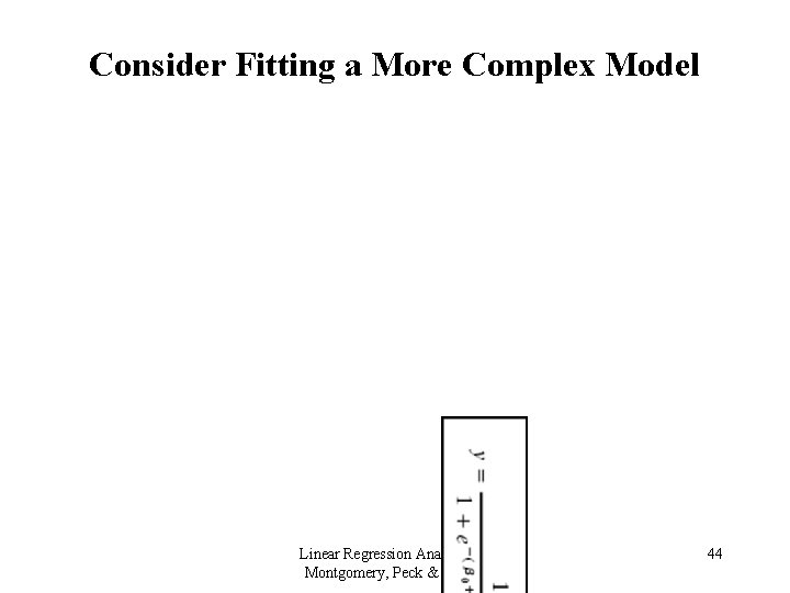
Consider Fitting a More Complex Model Linear Regression Analysis 5 E Montgomery, Peck & Vining 44

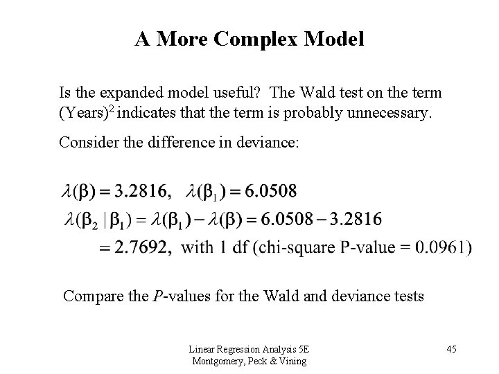
A More Complex Model Is the expanded model useful? The Wald test on the term (Years)2 indicates that the term is probably unnecessary. Consider the difference in deviance: Compare the P-values for the Wald and deviance tests Linear Regression Analysis 5 E Montgomery, Peck & Vining 45

Linear Regression Analysis 5 E Montgomery, Peck & Vining 46

Linear Regression Analysis 5 E Montgomery, Peck & Vining 47

Linear Regression Analysis 5 E Montgomery, Peck & Vining 48

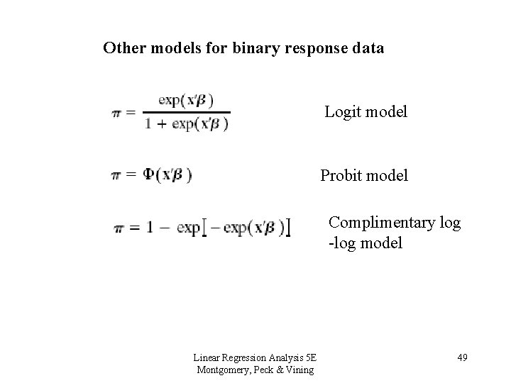
Other models for binary response data Logit model Probit model Complimentary log -log model Linear Regression Analysis 5 E Montgomery, Peck & Vining 49

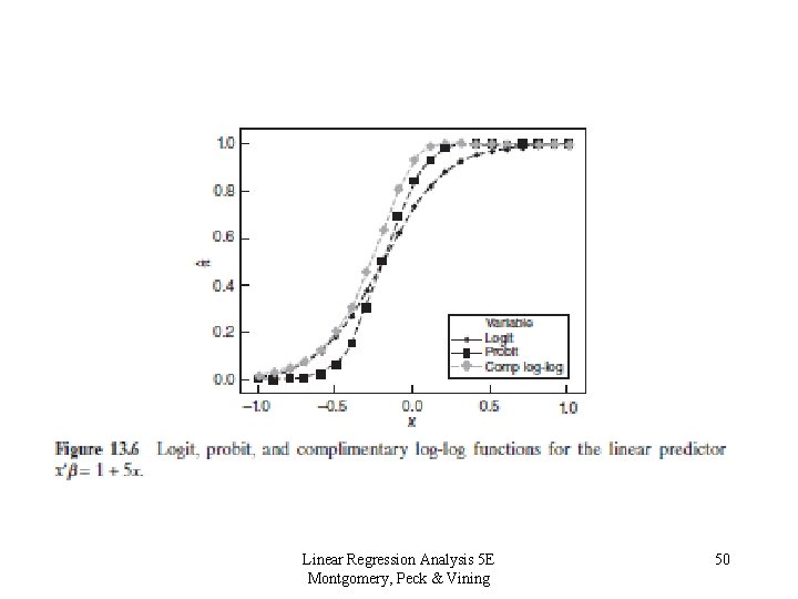
Linear Regression Analysis 5 E Montgomery, Peck & Vining 50

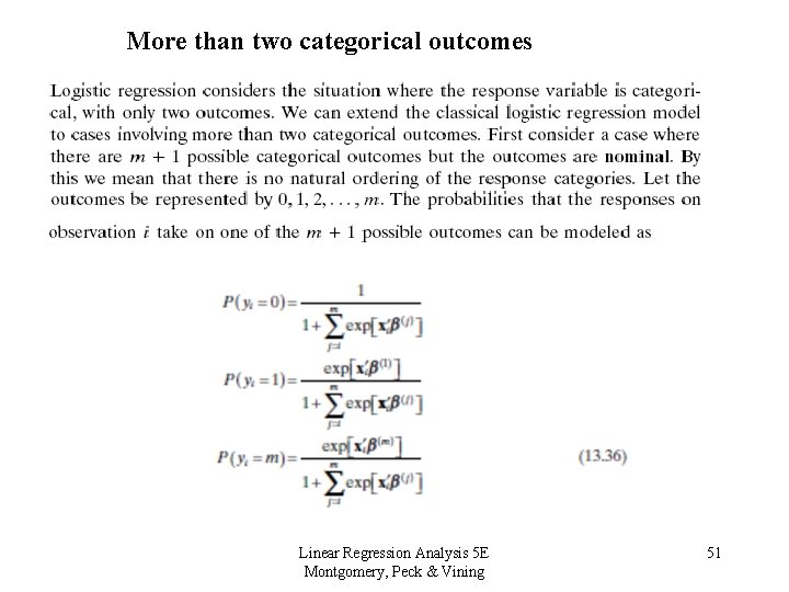
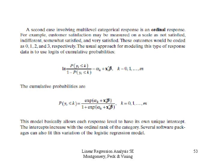
More than two categorical outcomes Linear Regression Analysis 5 E Montgomery, Peck & Vining 51

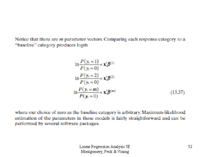
Linear Regression Analysis 5 E Montgomery, Peck & Vining 52

Linear Regression Analysis 5 E Montgomery, Peck & Vining 53

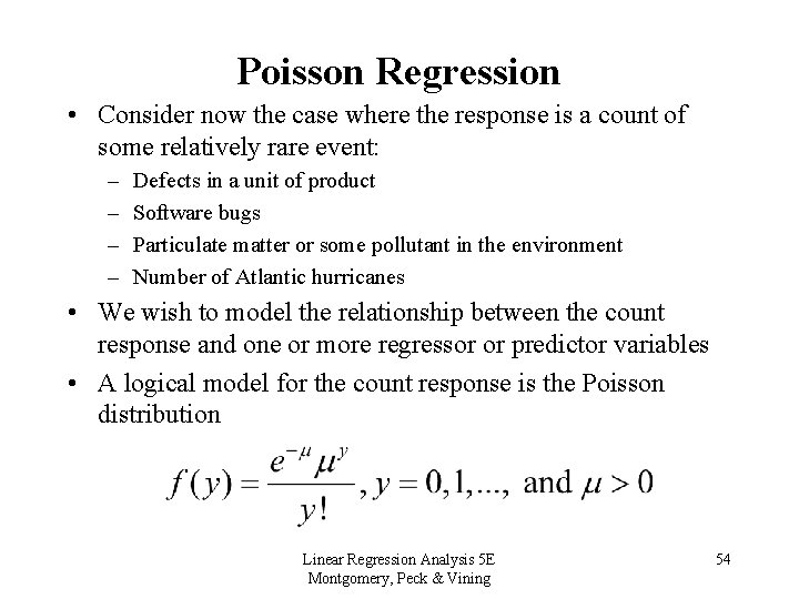
Poisson Regression • Consider now the case where the response is a count of some relatively rare event: – – Defects in a unit of product Software bugs Particulate matter or some pollutant in the environment Number of Atlantic hurricanes • We wish to model the relationship between the count response and one or more regressor or predictor variables • A logical model for the count response is the Poisson distribution Linear Regression Analysis 5 E Montgomery, Peck & Vining 54

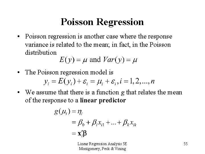
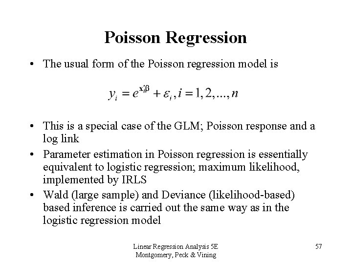
Poisson Regression • Poisson regression is another case where the response variance is related to the mean; in fact, in the Poisson distribution • The Poisson regression model is • We assume that there is a function g that relates the mean of the response to a linear predictor Linear Regression Analysis 5 E Montgomery, Peck & Vining 55

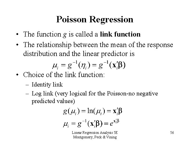
Poisson Regression • The function g is called a link function • The relationship between the mean of the response distribution and the linear predictor is • Choice of the link function: – Identity link – Log link (very logical for the Poisson-no negative predicted values) Linear Regression Analysis 5 E Montgomery, Peck & Vining 56

Poisson Regression • The usual form of the Poisson regression model is • This is a special case of the GLM; Poisson response and a log link • Parameter estimation in Poisson regression is essentially equivalent to logistic regression; maximum likelihood, implemented by IRLS • Wald (large sample) and Deviance (likelihood-based) based inference is carried out the same way as in the logistic regression model Linear Regression Analysis 5 E Montgomery, Peck & Vining 57

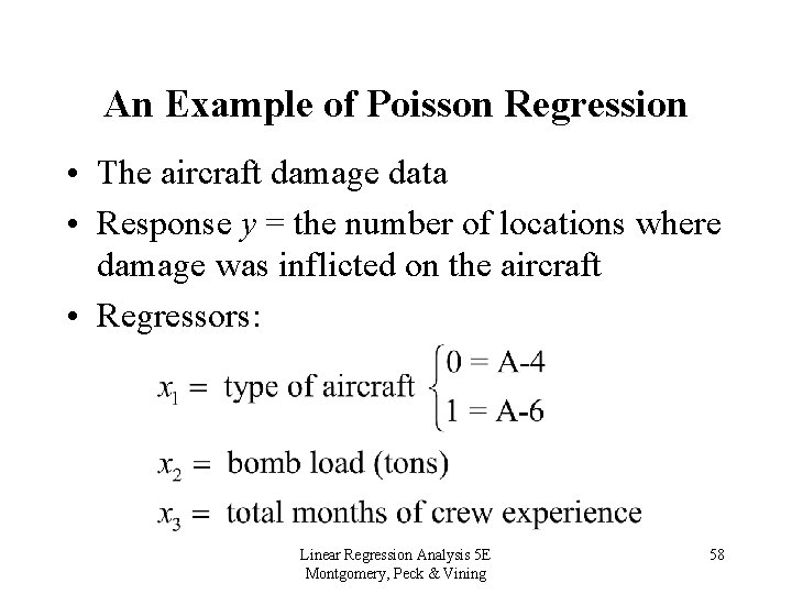
An Example of Poisson Regression • The aircraft damage data • Response y = the number of locations where damage was inflicted on the aircraft • Regressors: Linear Regression Analysis 5 E Montgomery, Peck & Vining 58

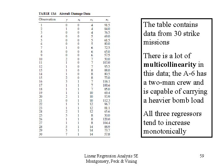
The table contains data from 30 strike missions There is a lot of multicollinearity in this data; the A-6 has a two-man crew and is capable of carrying a heavier bomb load All three regressors tend to increase monotonically Linear Regression Analysis 5 E Montgomery, Peck & Vining 59

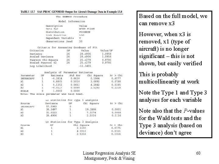
Based on the full model, we can remove x 3 However, when x 3 is removed, x 1 (type of aircraft) is no longer significant – this is not shown, but easily verified This is probably multicollinearity at work Note the Type 1 and Type 3 analyses for each variable Note also that the P-values for the Wald tests and the Type 3 analysis (based on deviance) don’t agree Linear Regression Analysis 5 E Montgomery, Peck & Vining 60

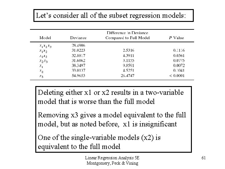
Let’s consider all of the subset regression models: Deleting either x 1 or x 2 results in a two-variable model that is worse than the full model Removing x 3 gives a model equivalent to the full model, but as noted before, x 1 is insignificant One of the single-variable models (x 2) is equivalent to the full model Linear Regression Analysis 5 E Montgomery, Peck & Vining 61

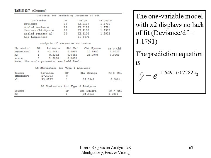
The one-variable model with x 2 displays no lack of fit (Deviance/df = 1. 1791) The prediction equation is Linear Regression Analysis 5 E Montgomery, Peck & Vining 62

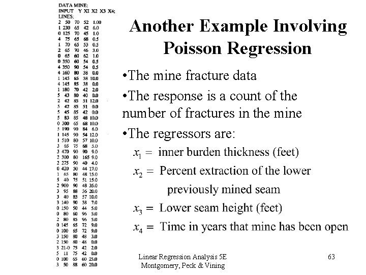
Another Example Involving Poisson Regression • The mine fracture data • The response is a count of the number of fractures in the mine • The regressors are: Linear Regression Analysis 5 E Montgomery, Peck & Vining 63

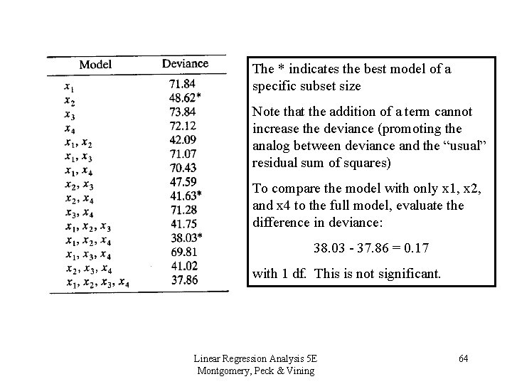
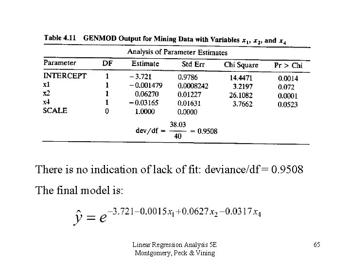
The * indicates the best model of a specific subset size Note that the addition of a term cannot increase the deviance (promoting the analog between deviance and the “usual” residual sum of squares) To compare the model with only x 1, x 2, and x 4 to the full model, evaluate the difference in deviance: 38. 03 - 37. 86 = 0. 17 with 1 df. This is not significant. Linear Regression Analysis 5 E Montgomery, Peck & Vining 64

There is no indication of lack of fit: deviance/df = 0. 9508 The final model is: Linear Regression Analysis 5 E Montgomery, Peck & Vining 65

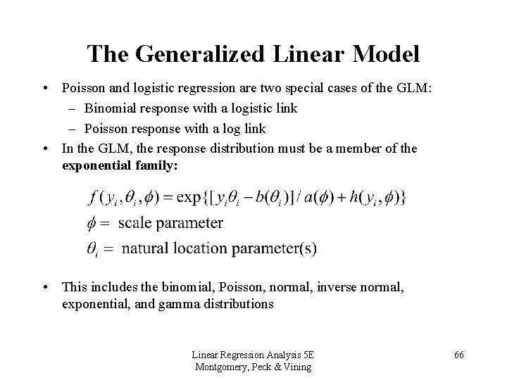
The Generalized Linear Model • Poisson and logistic regression are two special cases of the GLM: – Binomial response with a logistic link – Poisson response with a log link • In the GLM, the response distribution must be a member of the exponential family: • This includes the binomial, Poisson, normal, inverse normal, exponential, and gamma distributions Linear Regression Analysis 5 E Montgomery, Peck & Vining 66

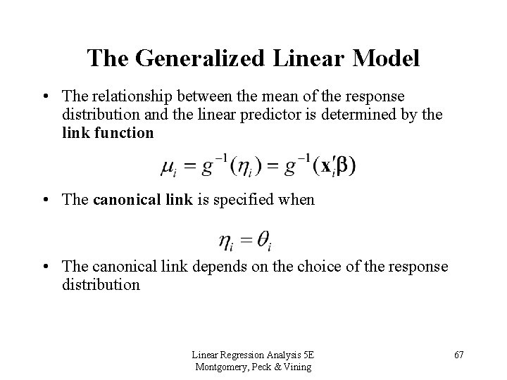
The Generalized Linear Model • The relationship between the mean of the response distribution and the linear predictor is determined by the link function • The canonical link is specified when • The canonical link depends on the choice of the response distribution Linear Regression Analysis 5 E Montgomery, Peck & Vining 67

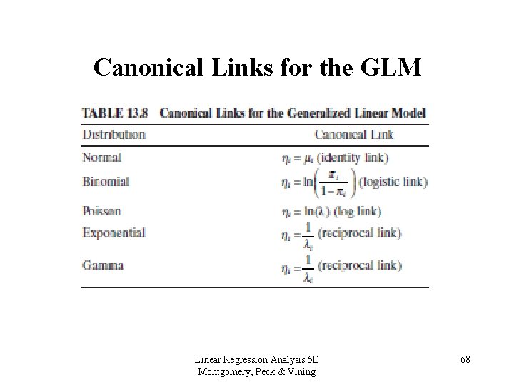
Canonical Links for the GLM Linear Regression Analysis 5 E Montgomery, Peck & Vining 68

Links for the GLM • You do not have to use the canonical link, it just simplifies some of the mathematics • In fact, the log (non-canonical) link is very often used with the exponential and gamma distributions, especially when the response variable is nonnegative • Other links can be based on the power family (as in power family transformations), or the complimentary log-log function Linear Regression Analysis 5 E Montgomery, Peck & Vining 69

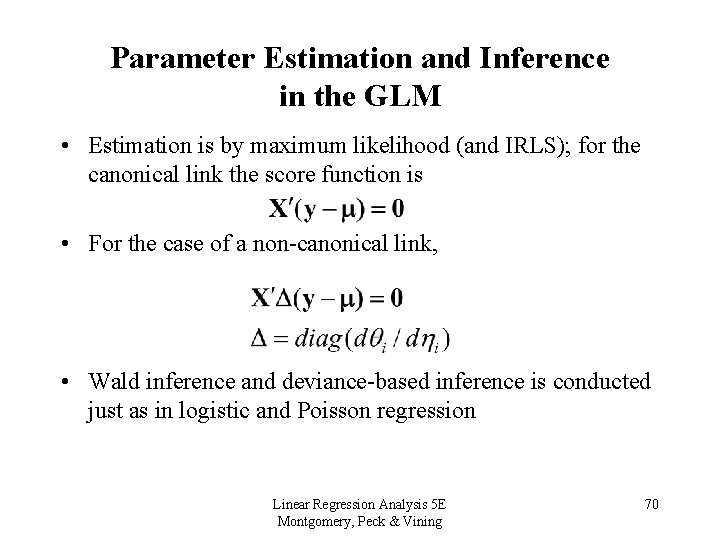
Parameter Estimation and Inference in the GLM • Estimation is by maximum likelihood (and IRLS); for the canonical link the score function is • For the case of a non-canonical link, • Wald inference and deviance-based inference is conducted just as in logistic and Poisson regression Linear Regression Analysis 5 E Montgomery, Peck & Vining 70

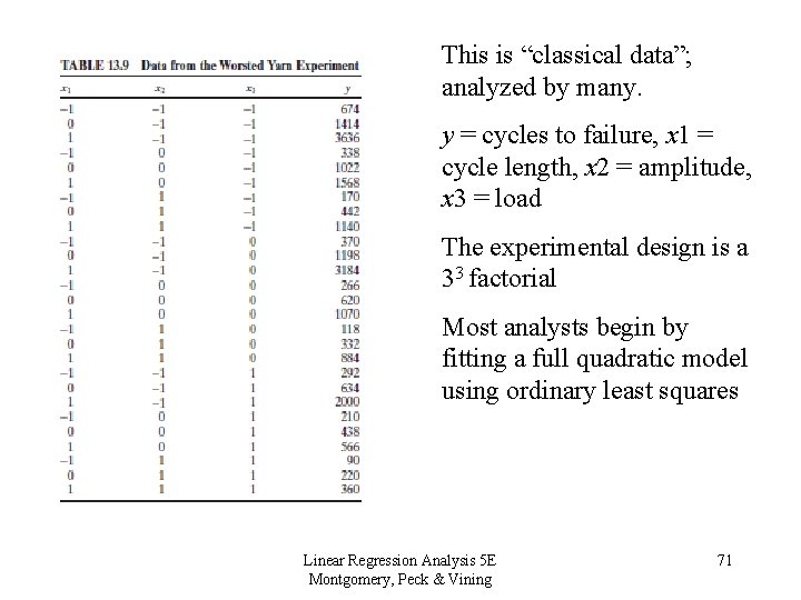
This is “classical data”; analyzed by many. y = cycles to failure, x 1 = cycle length, x 2 = amplitude, x 3 = load The experimental design is a 33 factorial Most analysts begin by fitting a full quadratic model using ordinary least squares Linear Regression Analysis 5 E Montgomery, Peck & Vining 71

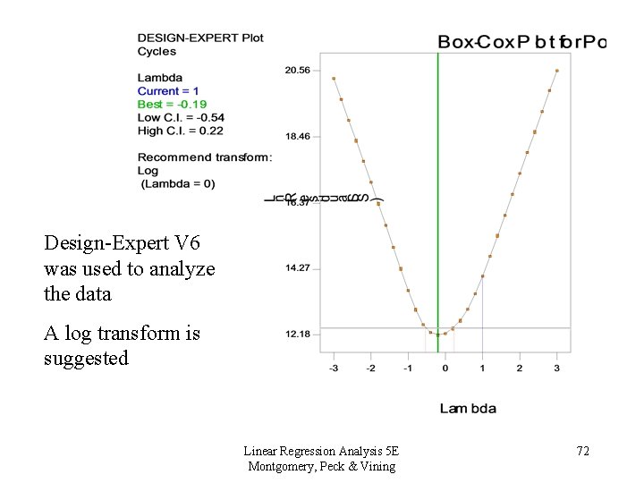
Design-Expert V 6 was used to analyze the data A log transform is suggested Linear Regression Analysis 5 E Montgomery, Peck & Vining 72

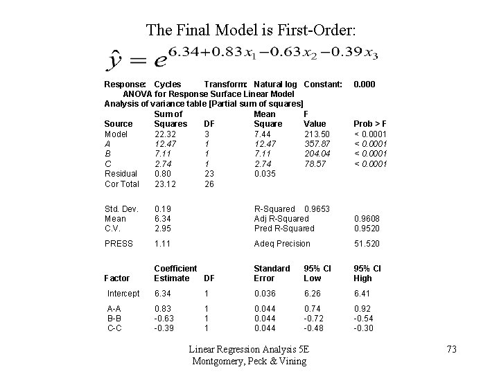
The Final Model is First-Order: Response: Cycles Transform: Natural log Constant: ANOVA for Response Surface Linear Model Analysis of variance table [Partial sum of squares] Sum of Mean F Source Squares DF Square Value Model 22. 32 3 7. 44 213. 50 A 12. 47 1 12. 47 357. 87 B 7. 11 1 7. 11 204. 04 C 2. 74 1 2. 74 78. 57 Residual 0. 80 23 0. 035 Cor Total 23. 12 26 0. 000 Prob > F < 0. 0001 Std. Dev. Mean C. V. 0. 19 6. 34 2. 95 R-Squared 0. 9653 Adj R-Squared Pred R-Squared 0. 9608 0. 9520 PRESS 1. 11 Adeq Precision 51. 520 Factor Coefficient Estimate DF Standard Error 95% CI Low 95% CI High Intercept 6. 34 1 0. 036 6. 26 6. 41 A-A B-B C-C 0. 83 -0. 63 -0. 39 1 1 1 0. 044 0. 74 -0. 72 -0. 48 0. 92 -0. 54 -0. 30 Linear Regression Analysis 5 E Montgomery, Peck & Vining 73

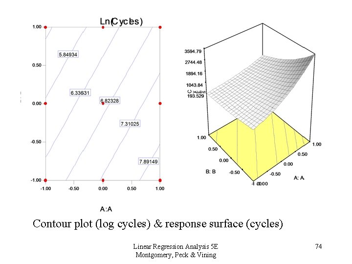
Contour plot (log cycles) & response surface (cycles) Linear Regression Analysis 5 E Montgomery, Peck & Vining 74

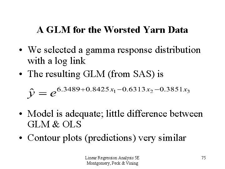
A GLM for the Worsted Yarn Data • We selected a gamma response distribution with a log link • The resulting GLM (from SAS) is • Model is adequate; little difference between GLM & OLS • Contour plots (predictions) very similar Linear Regression Analysis 5 E Montgomery, Peck & Vining 75

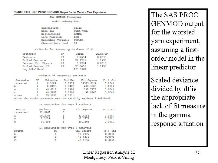
The SAS PROC GENMOD output for the worsted yarn experiment, assuming a firstorder model in the linear predictor Scaled deviance divided by df is the appropriate lack of fit measure in the gamma response situation Linear Regression Analysis 5 E Montgomery, Peck & Vining 76

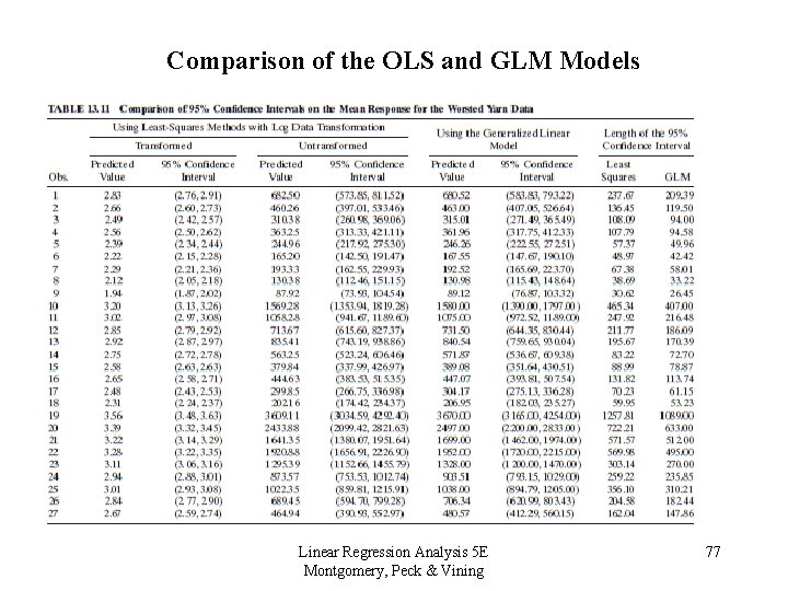
Comparison of the OLS and GLM Models Linear Regression Analysis 5 E Montgomery, Peck & Vining 77

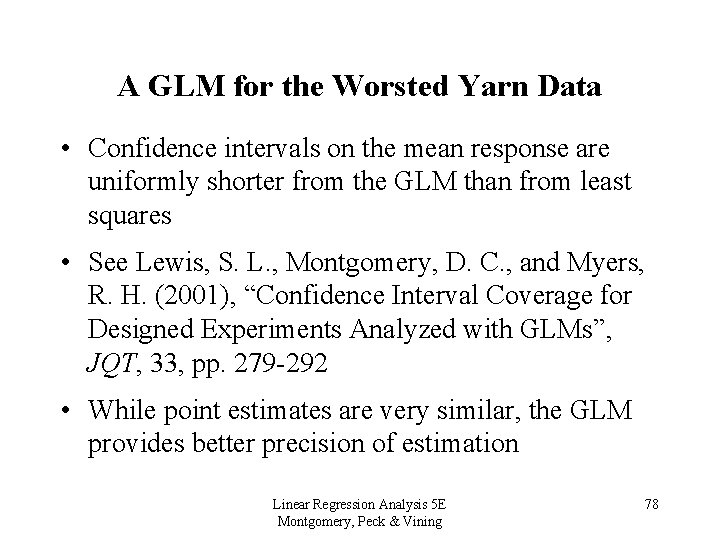
A GLM for the Worsted Yarn Data • Confidence intervals on the mean response are uniformly shorter from the GLM than from least squares • See Lewis, S. L. , Montgomery, D. C. , and Myers, R. H. (2001), “Confidence Interval Coverage for Designed Experiments Analyzed with GLMs”, JQT, 33, pp. 279 -292 • While point estimates are very similar, the GLM provides better precision of estimation Linear Regression Analysis 5 E Montgomery, Peck & Vining 78

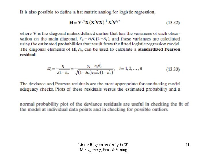
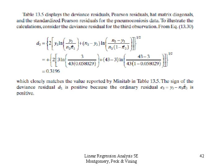
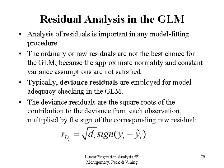
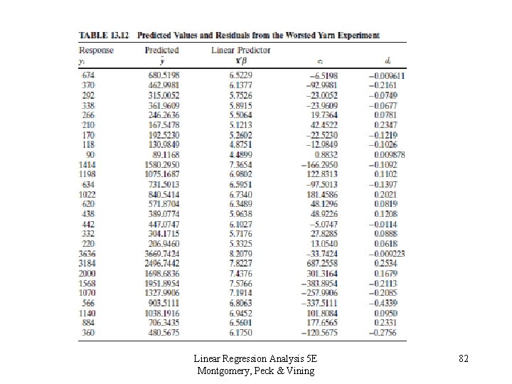
Residual Analysis in the GLM • Analysis of residuals is important in any model-fitting procedure • The ordinary or raw residuals are not the best choice for the GLM, because the approximate normality and constant variance assumptions are not satisfied • Typically, deviance residuals are employed for model adequacy checking in the GLM. • The deviance residuals are the square roots of the contribution to the deviance from each observation, multiplied by the sign of the corresponding raw residual: Linear Regression Analysis 5 E Montgomery, Peck & Vining 79

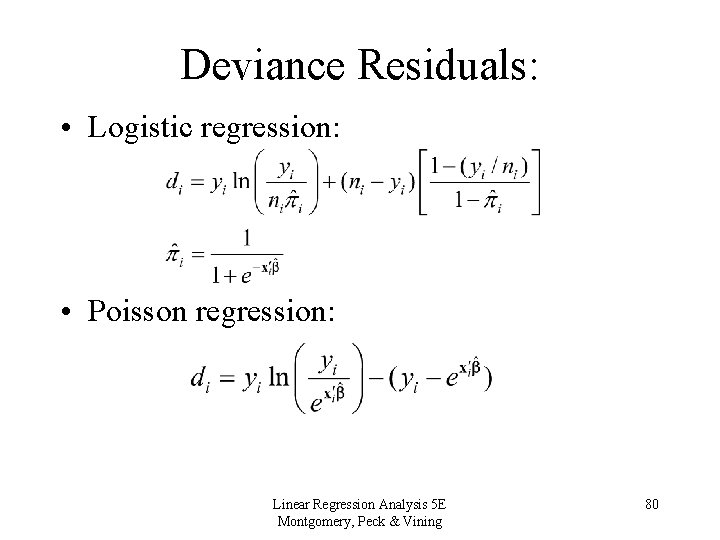
Deviance Residuals: • Logistic regression: • Poisson regression: Linear Regression Analysis 5 E Montgomery, Peck & Vining 80

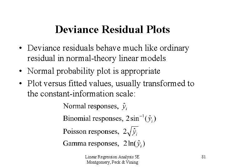
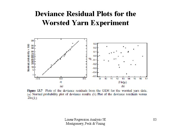
Deviance Residual Plots • Deviance residuals behave much like ordinary residual in normal-theory linear models • Normal probability plot is appropriate • Plot versus fitted values, usually transformed to the constant-information scale: Linear Regression Analysis 5 E Montgomery, Peck & Vining 81

Linear Regression Analysis 5 E Montgomery, Peck & Vining 82

Deviance Residual Plots for the Worsted Yarn Experiment Linear Regression Analysis 5 E Montgomery, Peck & Vining 83

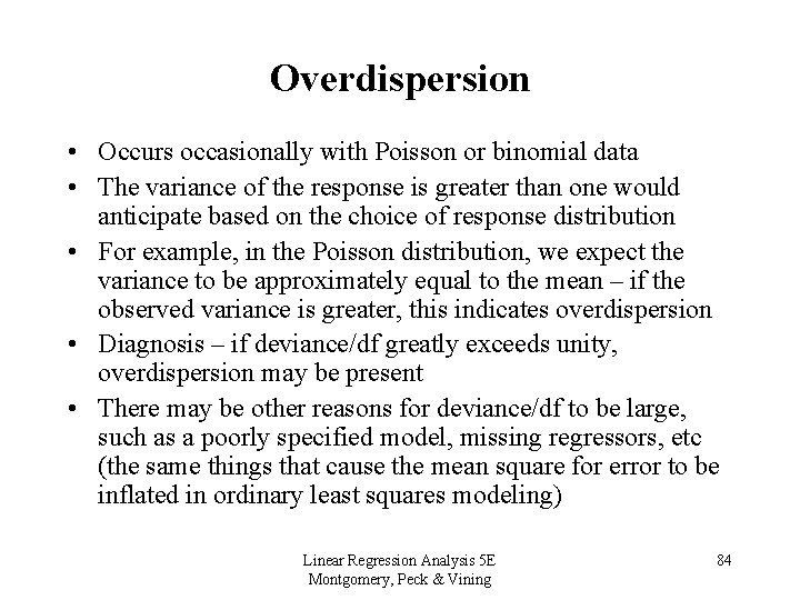
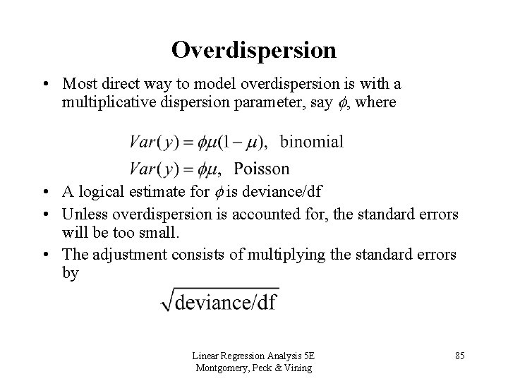
Overdispersion • Occurs occasionally with Poisson or binomial data • The variance of the response is greater than one would anticipate based on the choice of response distribution • For example, in the Poisson distribution, we expect the variance to be approximately equal to the mean – if the observed variance is greater, this indicates overdispersion • Diagnosis – if deviance/df greatly exceeds unity, overdispersion may be present • There may be other reasons for deviance/df to be large, such as a poorly specified model, missing regressors, etc (the same things that cause the mean square for error to be inflated in ordinary least squares modeling) Linear Regression Analysis 5 E Montgomery, Peck & Vining 84

Overdispersion • Most direct way to model overdispersion is with a multiplicative dispersion parameter, say , where • A logical estimate for is deviance/df • Unless overdispersion is accounted for, the standard errors will be too small. • The adjustment consists of multiplying the standard errors by Linear Regression Analysis 5 E Montgomery, Peck & Vining 85

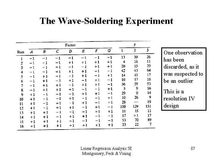
The Wave-Soldering Experiment • Response is the number of defects • Seven design variables: – – – – A = prebake condition B = flux denisty C = conveyor speed D = preheat condition E = cooling time F = ultrasonic solder agitator G = solder temperature Linear Regression Analysis 5 E Montgomery, Peck & Vining 86

The Wave-Soldering Experiment One observation has been discarded, as it was suspected to be an outlier This is a resolution IV design Linear Regression Analysis 5 E Montgomery, Peck & Vining 87

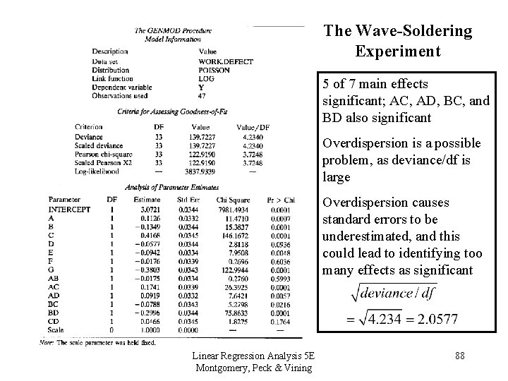
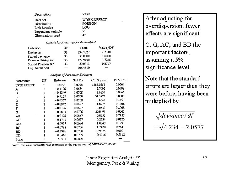
The Wave-Soldering Experiment 5 of 7 main effects significant; AC, AD, BC, and BD also significant Overdispersion is a possible problem, as deviance/df is large Overdispersion causes standard errors to be underestimated, and this could lead to identifying too many effects as significant Linear Regression Analysis 5 E Montgomery, Peck & Vining 88

After adjusting for overdispersion, fewer effects are significant C, G, AC, and BD the important factors, assuming a 5% significance level Note that the standard errors are larger than they were before, having been multiplied by Linear Regression Analysis 5 E Montgomery, Peck & Vining 89

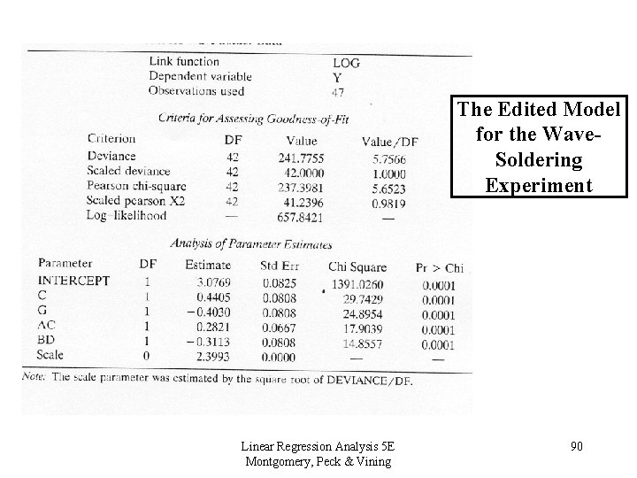
The Edited Model for the Wave. Soldering Experiment Linear Regression Analysis 5 E Montgomery, Peck & Vining 90

Generalized Linear Models • The GLM is a unification of linear and nonlinear models that can accommodate a wide variety of response distributions • Can be used with both regression models and designed experiments • Computer implementations in Minitab, JMP, SAS (PROC GENMOD), S-Plus • Logistic regression available in many basic packages • GLMs are a useful alternative to data transformation, and should always be considered when data transformations are not entirely satisfactory • Unlike data transformations, GLMs directly attack the unequal variance problem and use the maximum likelihood approach to account for the form of the response distribution Linear Regression Analysis 5 E Montgomery, Peck & Vining 91