Chapter 8 Trendlines and Regression Analysis Modeling Relationships

Chapter 8 Trendlines and Regression Analysis

Modeling Relationships and Trends in Data Create charts to better understand data sets. For cross-sectional data, use a scatter chart. For time series data, use a line chart.

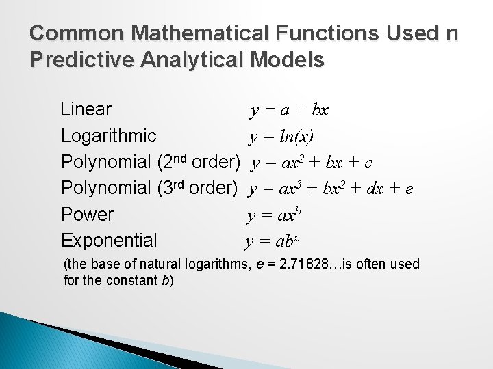
Common Mathematical Functions Used n Predictive Analytical Models Linear y = a + bx Logarithmic y = ln(x) Polynomial (2 nd order) y = ax 2 + bx + c Polynomial (3 rd order) y = ax 3 + bx 2 + dx + e Power y = axb Exponential y = abx (the base of natural logarithms, e = 2. 71828…is often used for the constant b)

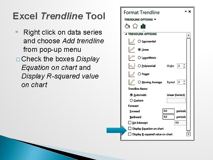
Excel Trendline Tool Right click on data series and choose Add trendline from pop-up menu � Check the boxes Display Equation on chart and Display R-squared value on chart

R 2 (R-squared) is a measure of the “fit” of the line to the data. ◦ The value of R 2 will be between 0 and 1. ◦ A value of 1. 0 indicates a perfect fit and all data points would lie on the line; the larger the value of R 2 the better the fit.

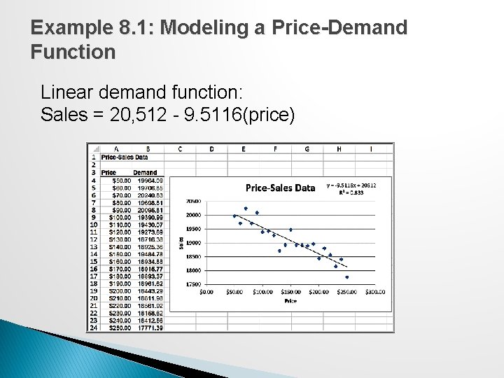
Example 8. 1: Modeling a Price-Demand Function Linear demand function: Sales = 20, 512 - 9. 5116(price)

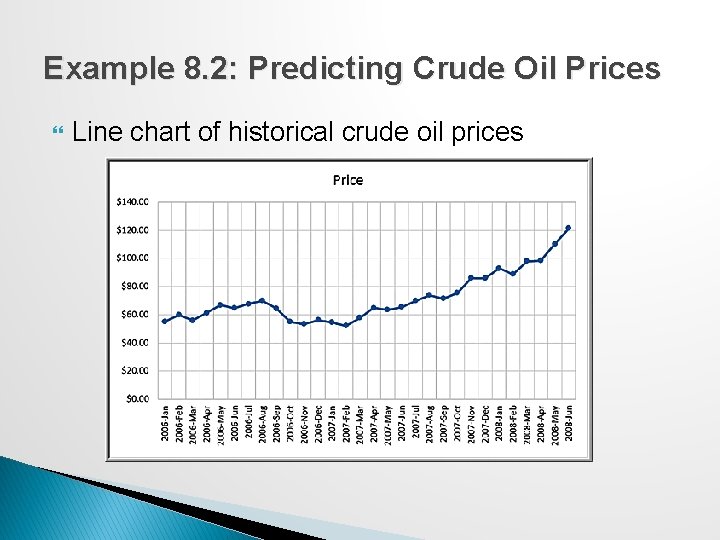
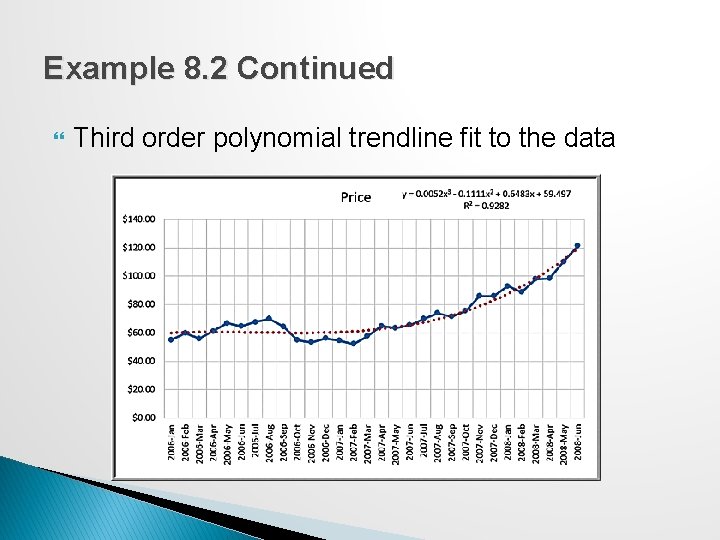
Example 8. 2: Predicting Crude Oil Prices Line chart of historical crude oil prices

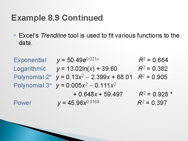
Example 8. 9 Continued Excel’s Trendline tool is used to fit various functions to the data. Exponential Logarithmic Polynomial 2° Polynomial 3° Power y = 50. 49 e 0. 021 x y = 13. 02 ln(x) + 39. 60 y = 0. 13 x 2 − 2. 399 x + 68. 01 y = 0. 005 x 3 − 0. 111 x 2 + 0. 648 x + 59. 497 y = 45. 96 x 0. 0169 R 2 = 0. 664 R 2 = 0. 382 R 2 = 0. 905 R 2 = 0. 928 * R 2 = 0. 397

Example 8. 2 Continued Third order polynomial trendline fit to the data Figure 8. 11

Caution About Polynomials The R 2 value will continue to increase as the order of the polynomial increases; that is, a 4 th order polynomial will provide a better fit than a 3 rd order, and so on. Higher order polynomials will generally not be very smooth and will be difficult to interpret visually. ◦ Thus, we don't recommend going beyond a third-order polynomial when fitting data. Use your eye to make a good judgment!

Regression Analysis Regression analysis is a tool for building mathematical and statistical models that characterize relationships between a dependent (ratio) variable and one or more independent, or explanatory variables (ratio or categorical), all of which are numerical. Simple linear regression involves a single independent variable. Multiple regression involves two or more independent variables.

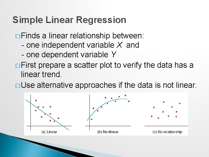
Simple Linear Regression � Finds a linear relationship between: - one independent variable X and - one dependent variable Y � First prepare a scatter plot to verify the data has a linear trend. � Use alternative approaches if the data is not linear.

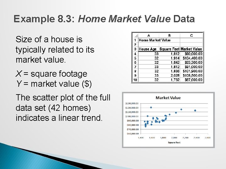
Example 8. 3: Home Market Value Data Size of a house is typically related to its market value. X = square footage Y = market value ($) The scatter plot of the full data set (42 homes) indicates a linear trend.

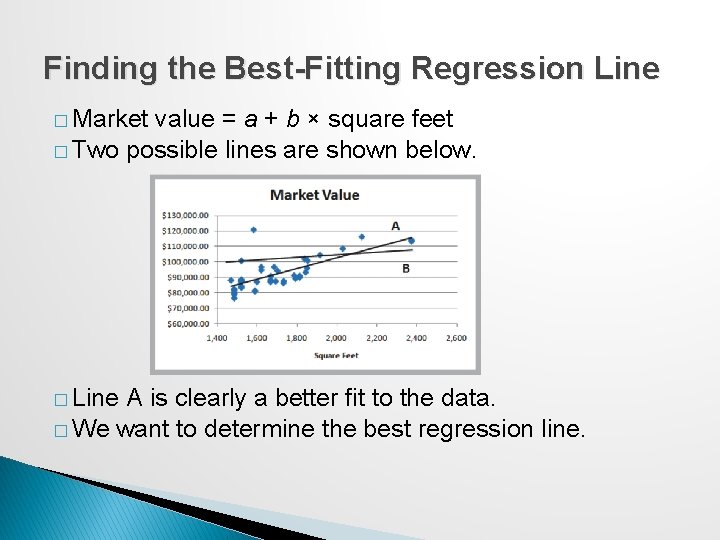
Finding the Best-Fitting Regression Line � Market value = a + b × square feet � Two possible lines are shown below. � Line A is clearly a better fit to the data. � We want to determine the best regression line.

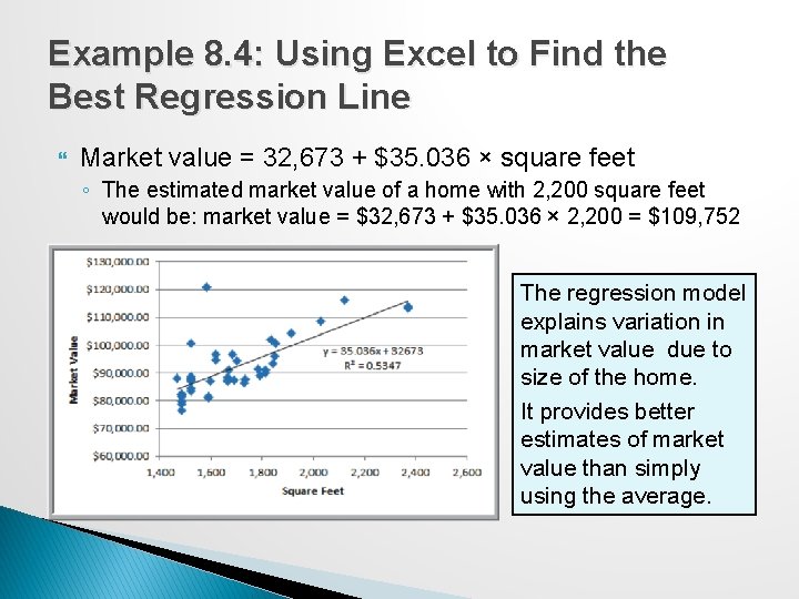
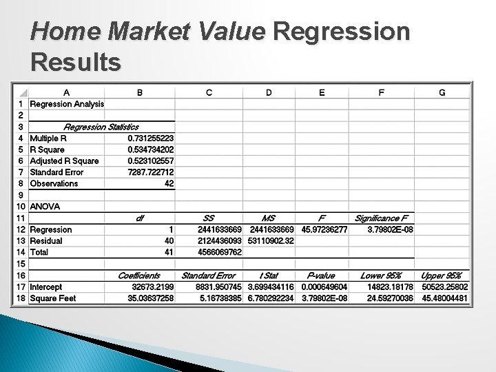
Example 8. 4: Using Excel to Find the Best Regression Line Market value = 32, 673 + $35. 036 × square feet ◦ The estimated market value of a home with 2, 200 square feet would be: market value = $32, 673 + $35. 036 × 2, 200 = $109, 752 The regression model explains variation in market value due to size of the home. It provides better estimates of market value than simply using the average.

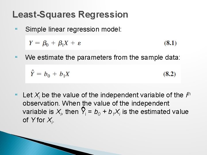
Least-Squares Regression Simple linear regression model: We estimate the parameters from the sample data: Let Xi be the value of the independent variable of the ith observation. When the value of the independent variable is Xi, then Yi = b 0 + b 1 Xi is the estimated value of Y for Xi.

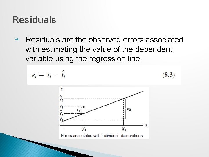
Residuals are the observed errors associated with estimating the value of the dependent variable using the regression line:

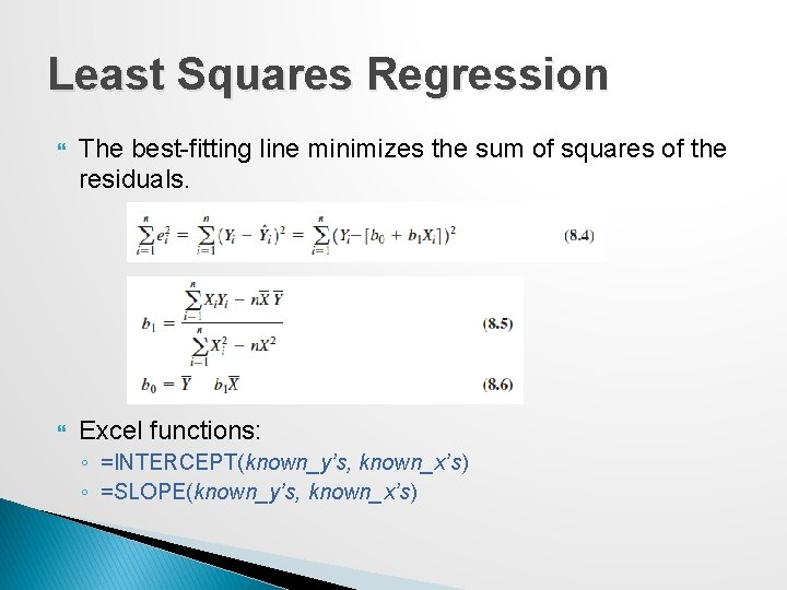
Least Squares Regression The best-fitting line minimizes the sum of squares of the residuals. Excel functions: ◦ =INTERCEPT(known_y’s, known_x’s) ◦ =SLOPE(known_y’s, known_x’s)

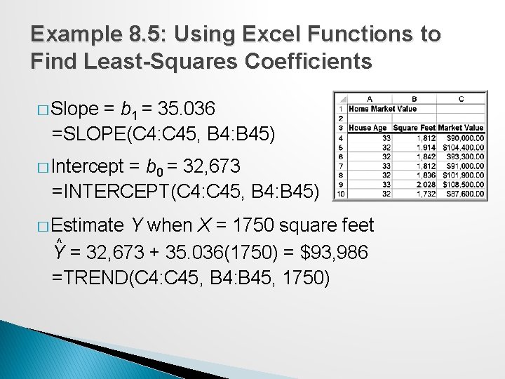
Example 8. 5: Using Excel Functions to Find Least-Squares Coefficients � Slope = b 1 = 35. 036 =SLOPE(C 4: C 45, B 4: B 45) � Intercept = b 0 = 32, 673 =INTERCEPT(C 4: C 45, B 4: B 45) � Estimate ^ Y when X = 1750 square feet Y = 32, 673 + 35. 036(1750) = $93, 986 =TREND(C 4: C 45, B 4: B 45, 1750)

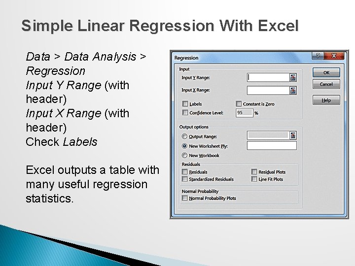
Simple Linear Regression With Excel Data > Data Analysis > Regression Input Y Range (with header) Input X Range (with header) Check Labels Excel outputs a table with many useful regression statistics.

Home Market Value Regression Results

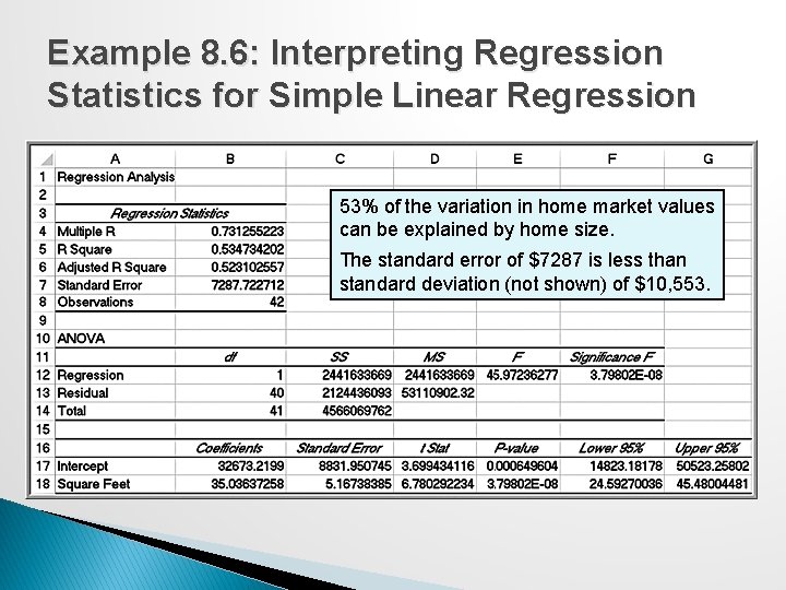
Regression Statistics � Multiple R - | r |, where r is the sample correlation coefficient. The value of r varies from -1 to +1 (r is negative if slope is negative) � R Square - coefficient of determination, R 2, which varies from 0 (no fit) to 1 (perfect fit) � Adjusted R Square - adjusts R 2 for sample size and number of X variables � Standard Error - variability between observed and predicted Y values. This is formally called the standard error of the estimate, SYX.

Example 8. 6: Interpreting Regression Statistics for Simple Linear Regression 53% of the variation in home market values can be explained by home size. The standard error of $7287 is less than standard deviation (not shown) of $10, 553.

Regression as Analysis of Variance ANOVA conducts an F-test to determine whether variation in Y is due to varying levels of X. ANOVA is used to test for significance of regression: H 0: population slope coefficient = 0 H 1: population slope coefficient ≠ 0 Excel reports the p-value (Significance F). Rejecting H 0 indicates that X explains variation in Y.

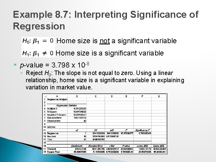
Example 8. 7: Interpreting Significance of Regression Home size is not a significant variable Home size is a significant variable p-value = 3. 798 x 10 -8 ◦ Reject H 0: The slope is not equal to zero. Using a linear relationship, home size is a significant variable in explaining variation in market value.

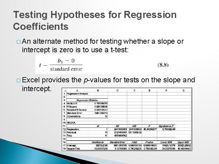
Testing Hypotheses for Regression Coefficients � An alternate method for testing whether a slope or intercept is zero is to use a t-test: � Excel provides the p-values for tests on the slope and intercept.

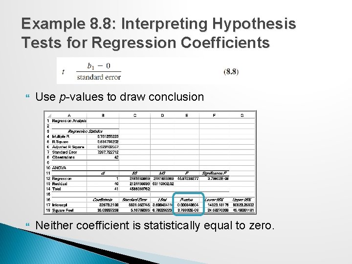
Example 8. 8: Interpreting Hypothesis Tests for Regression Coefficients Use p-values to draw conclusion Neither coefficient is statistically equal to zero.

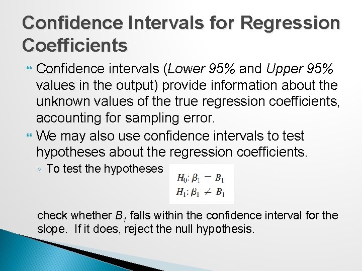
Confidence Intervals for Regression Coefficients Confidence intervals (Lower 95% and Upper 95% values in the output) provide information about the unknown values of the true regression coefficients, accounting for sampling error. We may also use confidence intervals to test hypotheses about the regression coefficients. ◦ To test the hypotheses check whether B 1 falls within the confidence interval for the slope. If it does, reject the null hypothesis.

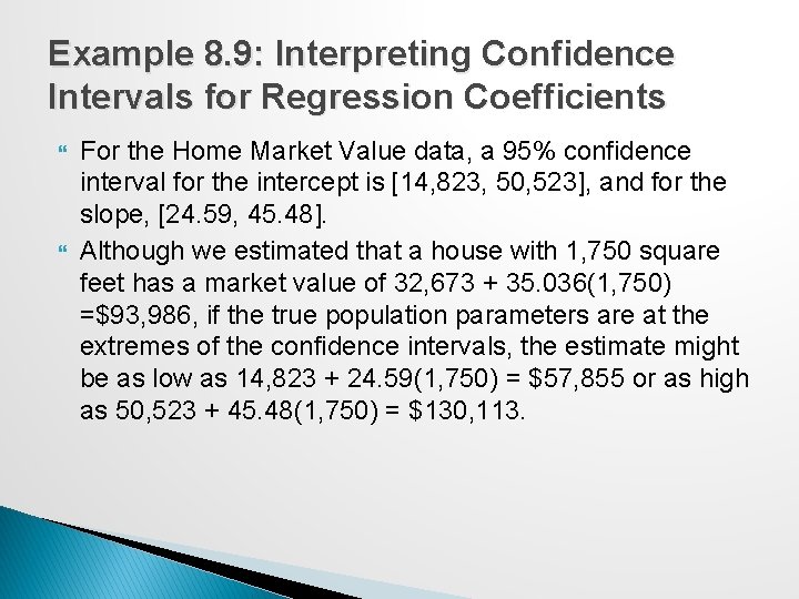
Example 8. 9: Interpreting Confidence Intervals for Regression Coefficients For the Home Market Value data, a 95% confidence interval for the intercept is [14, 823, 50, 523], and for the slope, [24. 59, 45. 48]. Although we estimated that a house with 1, 750 square feet has a market value of 32, 673 + 35. 036(1, 750) =$93, 986, if the true population parameters are at the extremes of the confidence intervals, the estimate might be as low as 14, 823 + 24. 59(1, 750) = $57, 855 or as high as 50, 523 + 45. 48(1, 750) = $130, 113.

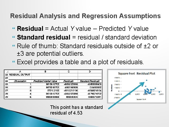
Residual Analysis and Regression Assumptions Residual = Actual Y value − Predicted Y value Standard residual = residual / standard deviation Rule of thumb: Standard residuals outside of ± 2 or ± 3 are potential outliers. Excel provides a table and a plot of residuals. This point has a standard residual of 4. 53

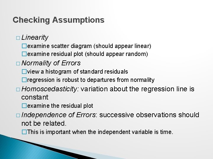
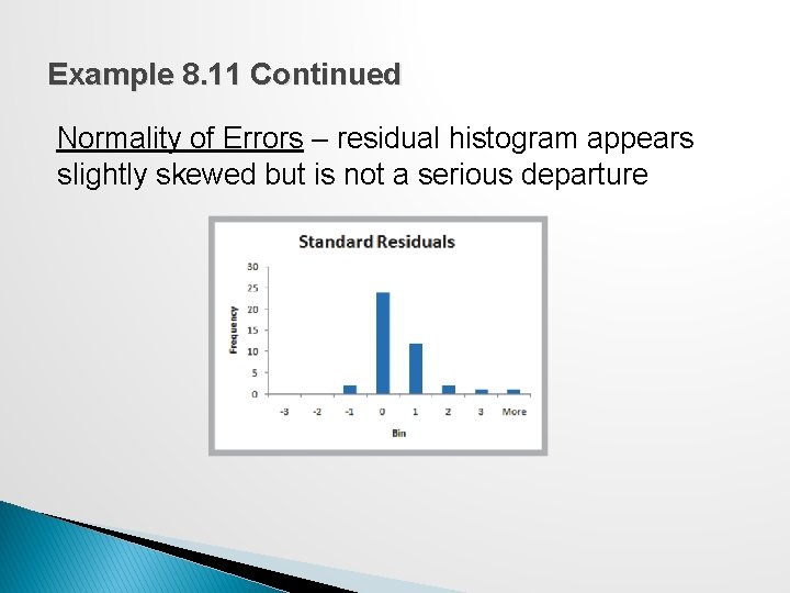
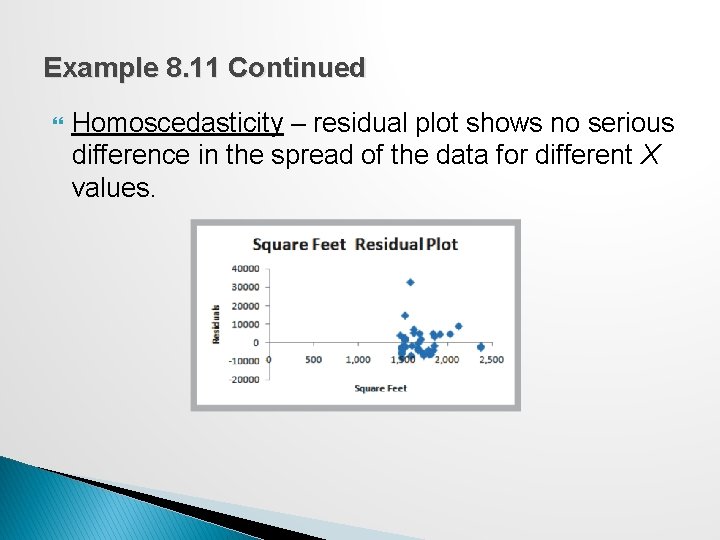
Checking Assumptions � Linearity �examine scatter diagram (should appear linear) �examine residual plot (should appear random) � Normality of Errors �view a histogram of standard residuals �regression is robust to departures from normality � Homoscedasticity: variation about the regression line is constant �examine the residual plot � Independence of Errors: successive observations should not be related. �This is important when the independent variable is time.

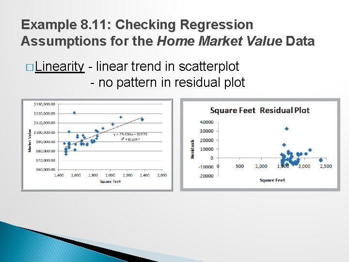
Example 8. 11: Checking Regression Assumptions for the Home Market Value Data � Linearity - linear trend in scatterplot - no pattern in residual plot

Example 8. 11 Continued Normality of Errors – residual histogram appears slightly skewed but is not a serious departure

Example 8. 11 Continued Homoscedasticity – residual plot shows no serious difference in the spread of the data for different X values.

Example 8. 11 Continued Independence of Errors – Because the data is cross-sectional, we can assume this assumption holds.

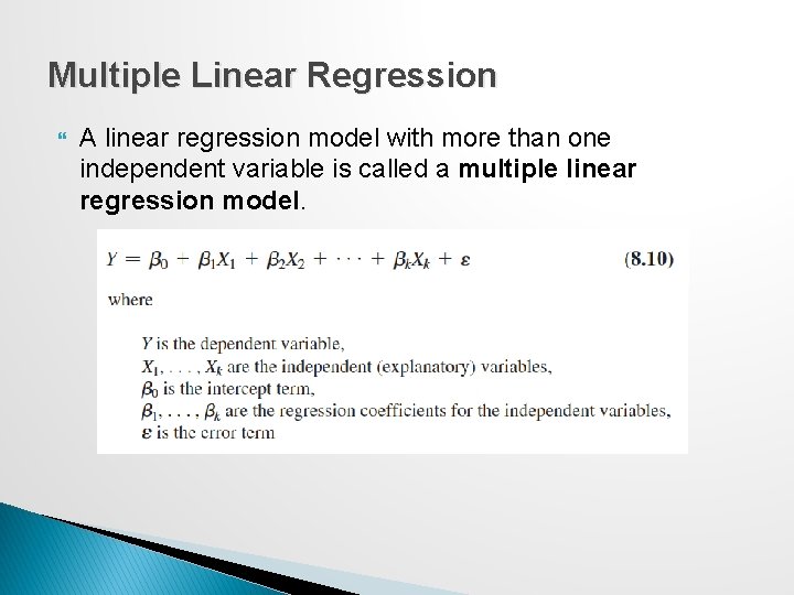
Multiple Linear Regression A linear regression model with more than one independent variable is called a multiple linear regression model.

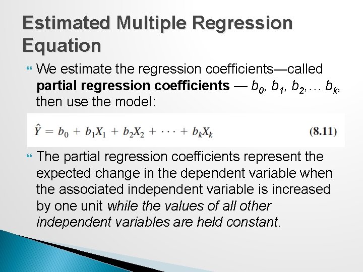
Estimated Multiple Regression Equation We estimate the regression coefficients—called partial regression coefficients — b 0, b 1, b 2, … bk, then use the model: The partial regression coefficients represent the expected change in the dependent variable when the associated independent variable is increased by one unit while the values of all other independent variables are held constant.

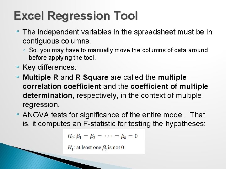
Excel Regression Tool The independent variables in the spreadsheet must be in contiguous columns. ◦ So, you may have to manually move the columns of data around before applying the tool. Key differences: Multiple R and R Square called the multiple correlation coefficient and the coefficient of multiple determination, respectively, in the context of multiple regression. ANOVA tests for significance of the entire model. That is, it computes an F-statistic for testing the hypotheses:

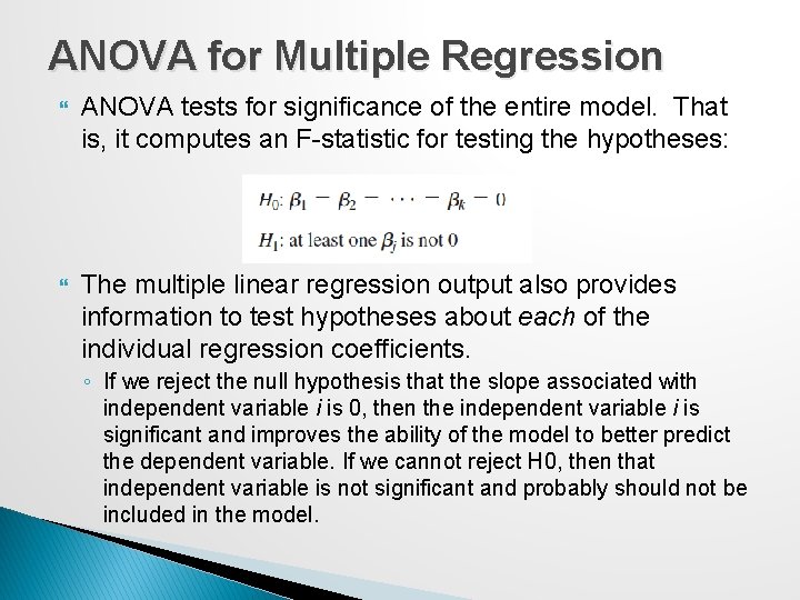
ANOVA for Multiple Regression ANOVA tests for significance of the entire model. That is, it computes an F-statistic for testing the hypotheses: The multiple linear regression output also provides information to test hypotheses about each of the individual regression coefficients. ◦ If we reject the null hypothesis that the slope associated with independent variable i is 0, then the independent variable i is significant and improves the ability of the model to better predict the dependent variable. If we cannot reject H 0, then that independent variable is not significant and probably should not be included in the model.

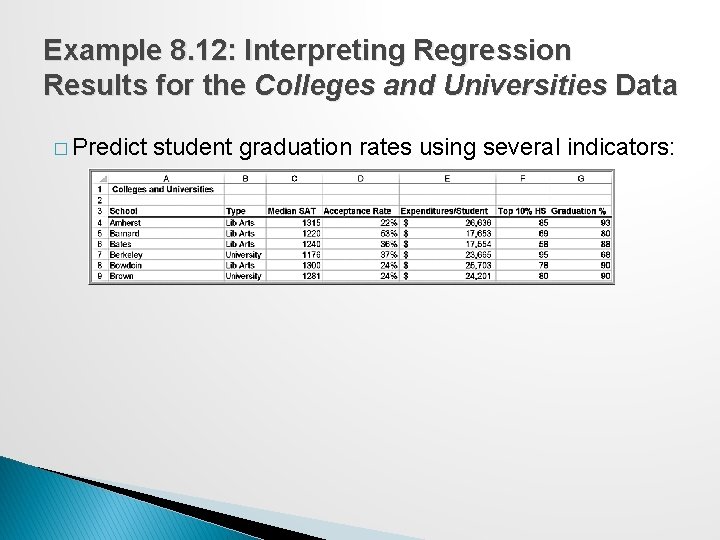
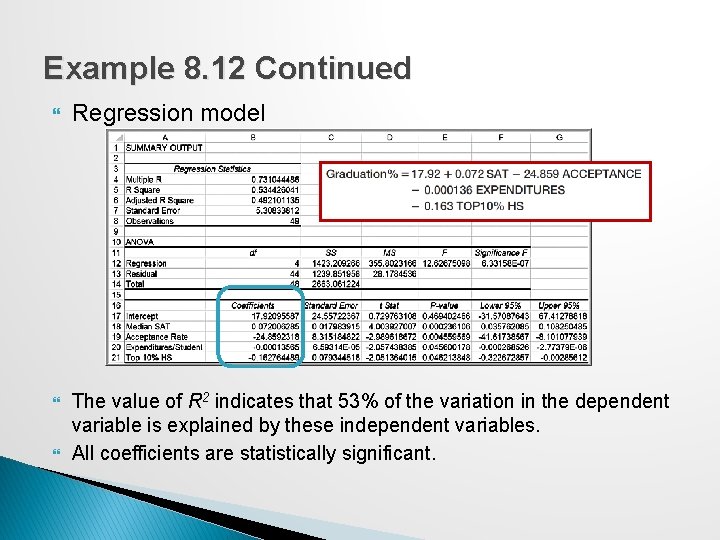
Example 8. 12: Interpreting Regression Results for the Colleges and Universities Data � Predict student graduation rates using several indicators:

Example 8. 12 Continued Regression model The value of R 2 indicates that 53% of the variation in the dependent variable is explained by these independent variables. All coefficients are statistically significant.

Model Building Issues A good regression model should include only significant independent variables. However, it is not always clear exactly what will happen when we add or remove variables from a model; variables that are (or are not) significant in one model may (or may not) be significant in another. ◦ Therefore, you should not consider dropping all insignificant variables at one time, but rather take a more structured approach. Adding an independent variable to a regression model will always result in R 2 equal to or greater than the R 2 of the original model. Adjusted R 2 reflects both the number of independent variables and the sample size and may either increase or decrease when an independent variable is added or dropped. An increase in adjusted R 2 indicates that the model has improved.

Systematic Model Building Approach 1. 2. 3. Construct a model with all available independent variables. Check for significance of the independent variables by examining the p-values. Identify the independent variable having the largest pvalue that exceeds the chosen level of significance. Remove the variable identified in step 2 from the model and evaluate adjusted R 2. (Don’t remove all variables with p-values that exceed a at the same time, but remove only one at a time. ) 4. Continue until all variables are significant.

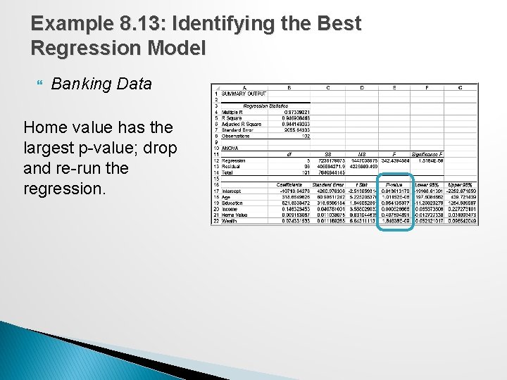
Example 8. 13: Identifying the Best Regression Model Banking Data Home value has the largest p-value; drop and re-run the regression.

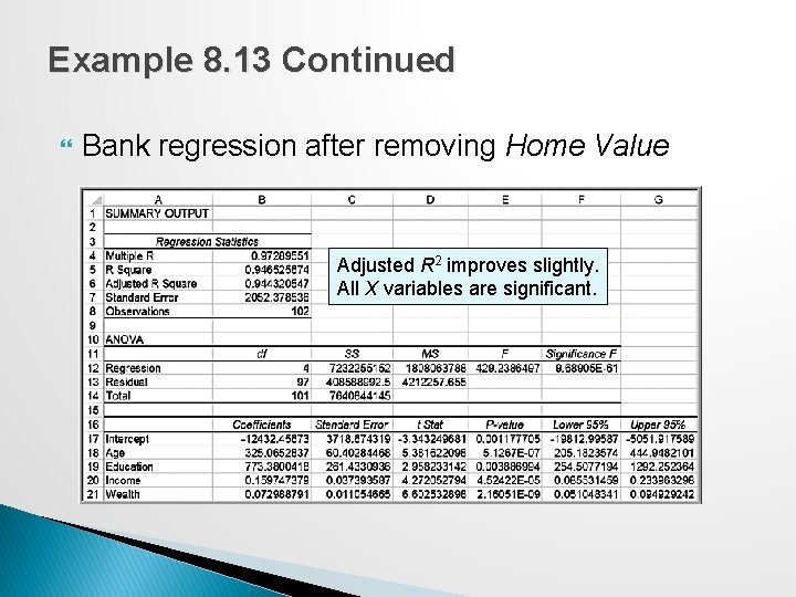
Example 8. 13 Continued Bank regression after removing Home Value Adjusted R 2 improves slightly. All X variables are significant.

Alternate Criterion Use the t-statistic. If | t | < 1, then the standard error will decrease and adjusted R 2 will increase if the variable is removed. If | t | > 1, then the opposite will occur. You can follow the same systematic approach, except using t-values instead of p-values.

Multicollinearity occurs when there are strong correlations among the independent variables, and they can predict each other better than the dependent variable. ◦ When significant multicollinearity is present, it becomes difficult to isolate the effect of one independent variable on the dependent variable, the signs of coefficients may be the opposite of what they should be, making it difficult to interpret regression coefficients, and p-values can be inflated. Correlations exceeding ± 0. 7 may indicate multicollinearity � The variance inflation factor is a better indicator, but not computed in Excel.

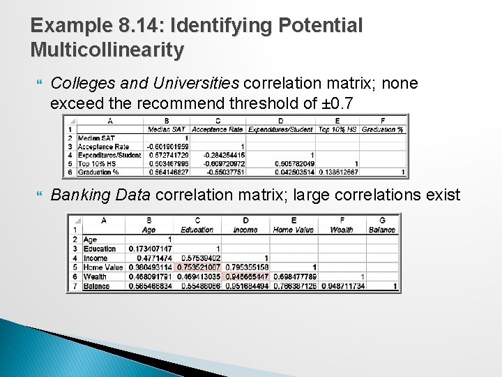
Example 8. 14: Identifying Potential Multicollinearity Colleges and Universities correlation matrix; none exceed the recommend threshold of ± 0. 7 Banking Data correlation matrix; large correlations exist

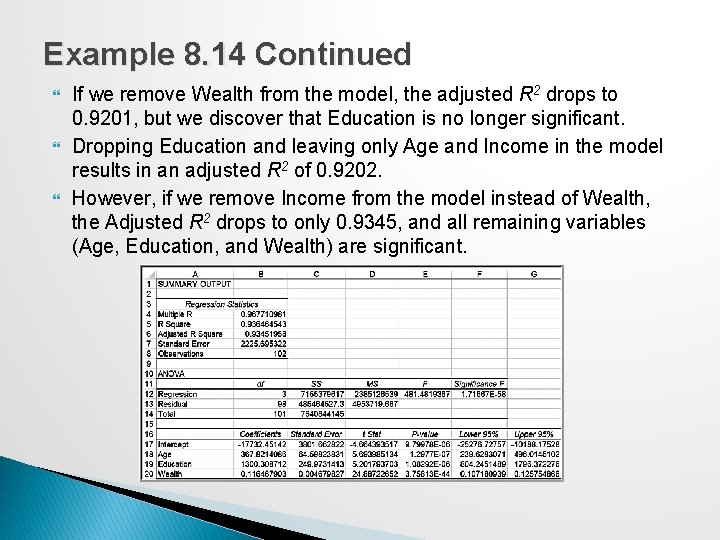
Example 8. 14 Continued If we remove Wealth from the model, the adjusted R 2 drops to 0. 9201, but we discover that Education is no longer significant. Dropping Education and leaving only Age and Income in the model results in an adjusted R 2 of 0. 9202. However, if we remove Income from the model instead of Wealth, the Adjusted R 2 drops to only 0. 9345, and all remaining variables (Age, Education, and Wealth) are significant.

Practical Issues in Trendline and Regression Modeling Identifying the best regression model often requires experimentation and trial and error. The independent variables selected should make sense in attempting to explain the dependent variable ◦ Logic should guide your model development. In many applications, behavioral, economic, or physical theory might suggest that certain variables should belong in a model. Additional variables increase R 2 and, therefore, help to explain a larger proportion of the variation. ◦ Even though a variable with a large p-value is not statistically significant, it could simply be the result of sampling error and a modeler might wish to keep it. Good models are as simple as possible (the principle of parsimony).

Overfitting means fiting a model too closely to the sample data at the risk of not fitting it well to the population in which we are interested. ◦ In fitting the crude oil prices in Example 8. 2, we noted that the R 2 value will increase if we fit higher-order polynomial functions to the data. While this might provide a better mathematical fit to the sample data, doing so can make it difficult to explain the phenomena rationally. In multiple regression, if we add too many terms to the model, then the model may not adequately predict other values from the population. Overfitting can be mitigated by using good logic, intuition, theory, and parsimony.

Regression with Categorical Variables Regression analysis requires numerical data. Categorical data can be included as independent variables, but must be coded numeric using dummy variables. � For variables with 2 categories, code as 0 and 1.

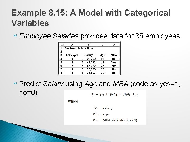
Example 8. 15: A Model with Categorical Variables Employee Salaries provides data for 35 employees Predict Salary using Age and MBA (code as yes=1, no=0)

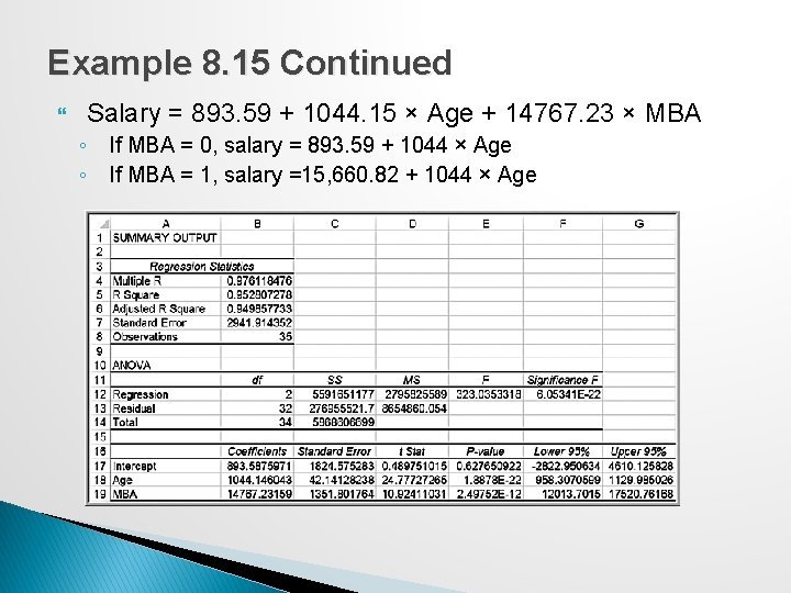
Example 8. 15 Continued Salary = 893. 59 + 1044. 15 × Age + 14767. 23 × MBA ◦ If MBA = 0, salary = 893. 59 + 1044 × Age ◦ If MBA = 1, salary =15, 660. 82 + 1044 × Age

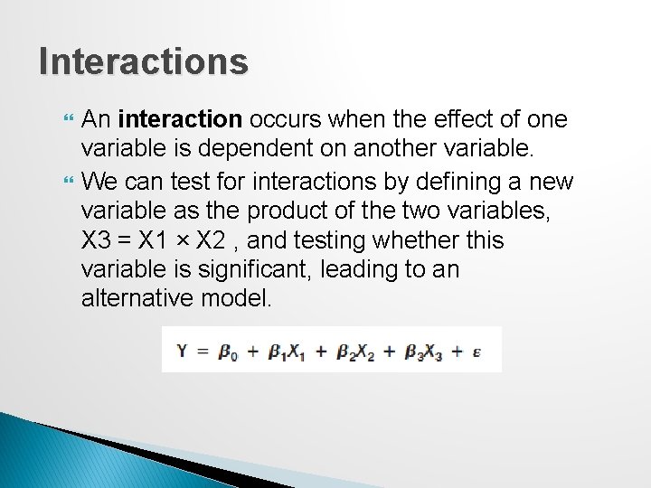
Interactions An interaction occurs when the effect of one variable is dependent on another variable. We can test for interactions by defining a new variable as the product of the two variables, X 3 = X 1 × X 2 , and testing whether this variable is significant, leading to an alternative model.

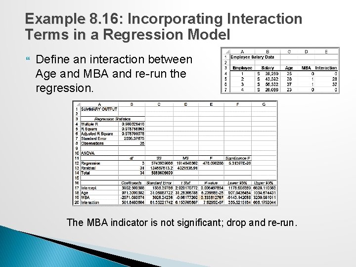
Example 8. 16: Incorporating Interaction Terms in a Regression Model Define an interaction between Age and MBA and re-run the regression. The MBA indicator is not significant; drop and re-run.

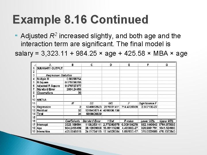
Example 8. 16 Continued Adjusted R 2 increased slightly, and both age and the interaction term are significant. The final model is salary = 3, 323. 11 + 984. 25 × age + 425. 58 × MBA × age

Categorical Variables with More Than Two Levels When a categorical variable has k > 2 levels, we need to add k - 1 additional variables to the model.

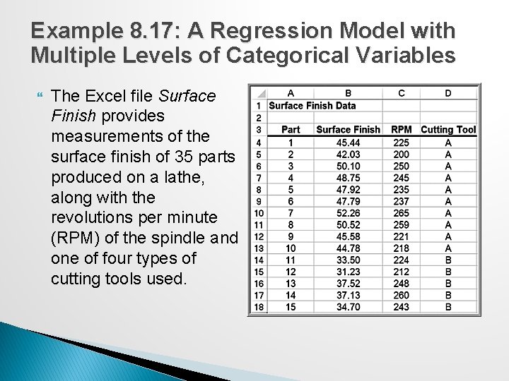
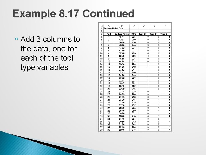
Example 8. 17: A Regression Model with Multiple Levels of Categorical Variables The Excel file Surface Finish provides measurements of the surface finish of 35 parts produced on a lathe, along with the revolutions per minute (RPM) of the spindle and one of four types of cutting tools used.

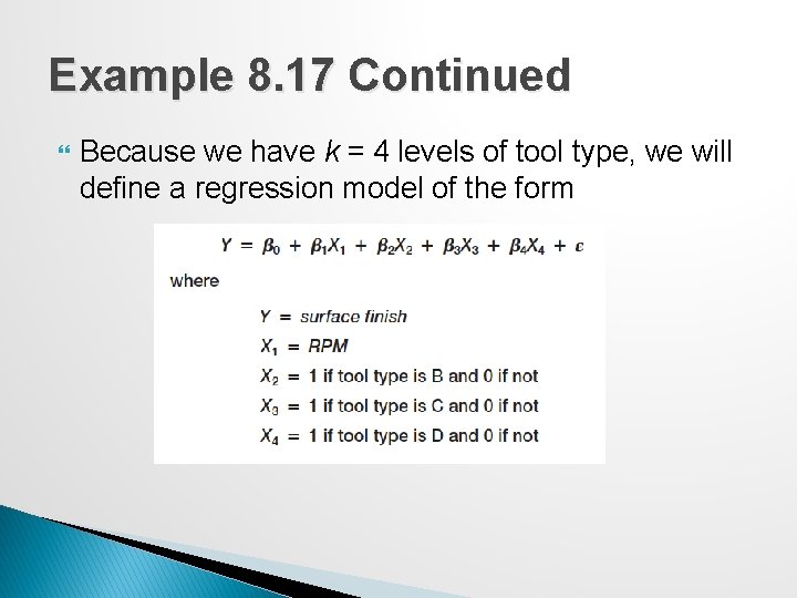
Example 8. 17 Continued Because we have k = 4 levels of tool type, we will define a regression model of the form

Example 8. 17 Continued Add 3 columns to the data, one for each of the tool type variables

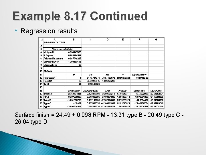
Example 8. 17 Continued Regression results Surface finish = 24. 49 + 0. 098 RPM - 13. 31 type B - 20. 49 type C 26. 04 type D

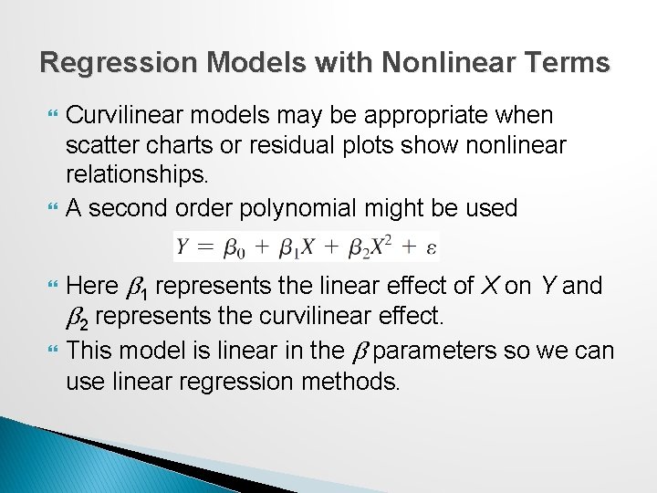
Regression Models with Nonlinear Terms Curvilinear models may be appropriate when scatter charts or residual plots show nonlinear relationships. A second order polynomial might be used Here β 1 represents the linear effect of X on Y and β 2 represents the curvilinear effect. This model is linear in the β parameters so we can use linear regression methods.

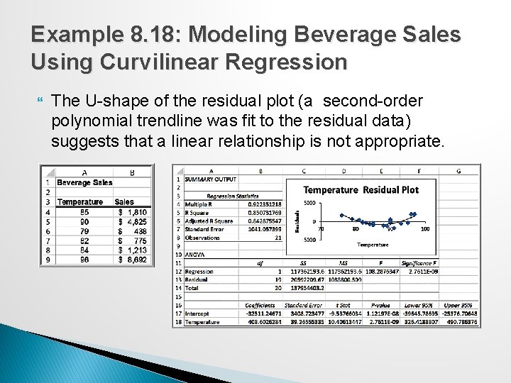
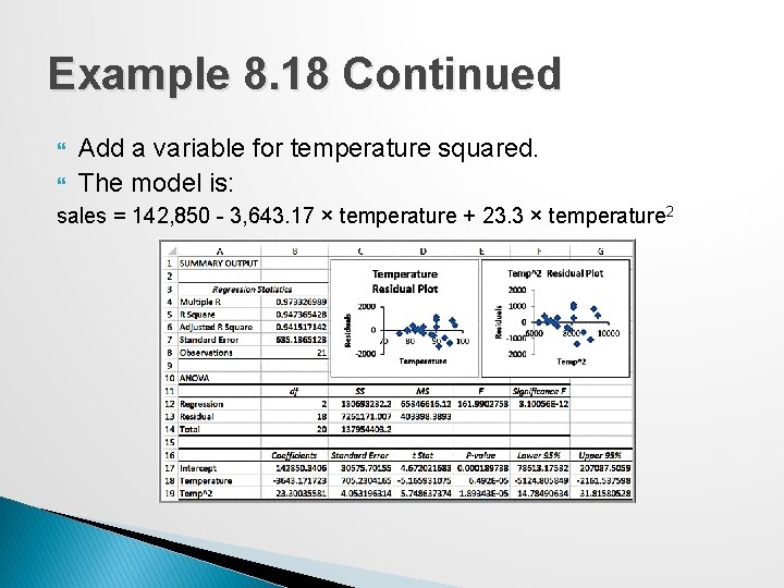
Example 8. 18: Modeling Beverage Sales Using Curvilinear Regression The U-shape of the residual plot (a second-order polynomial trendline was fit to the residual data) suggests that a linear relationship is not appropriate.

Example 8. 18 Continued Add a variable for temperature squared. The model is: sales = 142, 850 - 3, 643. 17 × temperature + 23. 3 × temperature 2

Advanced Techniques for Regression Modeling using XLMiner The regression analysis tool in XLMiner has some advanced options not available in Excel’s Descriptive Statistics tool. Best-subsets regression evaluates either all possible regression models for a set of independent variables or the best subsets of models for a fixed number of independent variables.

Evaluating Best Subsets Models Best subsets evaluates models using a statistic called Cp, (the Bonferroni criterion). ◦ Cp estimates the bias introduced in the estimates of the responses by having an underspecified model (a model with important predictors missing). ◦ If Cp is much greater than (the number of independent variables plus 1), there is substantial bias. The full model always has Cp = k + 1. ◦ If all models except the full model have large Cps, it suggests that important predictor variables are missing. Models with a minimum value or having Cp less than or at least close to are good models to consider.

Best-Subsets Procedures Backward Elimination begins with all independent variables in the model and deletes one at a time until the best model is identified. Forward Selection begins with a model having no independent variables and successively adds one at a time until no additional variable makes a significant contribution. Stepwise Selection is similar to Forward Selection except that at each step, the procedure considers dropping variables that are not statistically significant. Sequential Replacement replaces variables sequentially, retaining those that improve performance. These options might terminate with a different model. Exhaustive Search looks at all combinations of variables to find the one with the best fit, but it can be time consuming for large numbers of variables. 9 -68

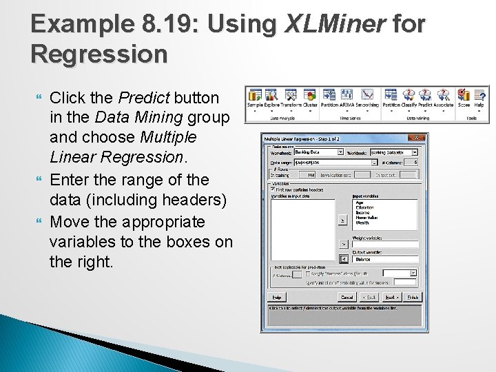
Example 8. 19: Using XLMiner for Regression Click the Predict button in the Data Mining group and choose Multiple Linear Regression. Enter the range of the data (including headers) Move the appropriate variables to the boxes on the right.

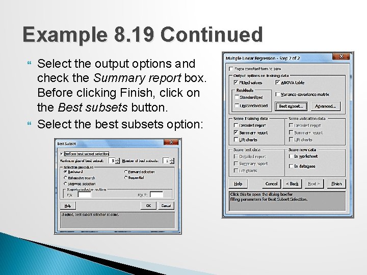
Example 8. 19 Continued Select the output options and check the Summary report box. Before clicking Finish, click on the Best subsets button. Select the best subsets option:

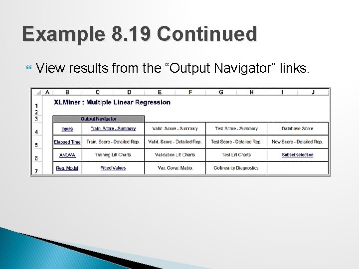
Example 8. 19 Continued View results from the “Output Navigator” links.

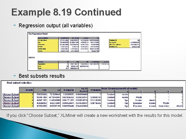
Example 8. 19 Continued Regression output (all variables) Best subsets results If you click “Choose Subset, ” XLMiner will create a new worksheet with the results for this model.

Interpreting XLMiner Output Typically choose the model with the highest adjusted R 2. Models with a minimum value of Cp or having Cp less than or at least close to k + 1 are good models to consider. RSS is the residual sum of squares, or the sum of squared deviations between the predicted probability of success and the actual value (1 or 0). Probability is a quasi-hypothesis test that a given subset is acceptable; if this is less than 0. 05, you can rule out that subset.