Regression Analysis AGEC 784 7 1 Modeling Relationships

Regression Analysis AGEC 784 7 -1

Modeling Relationships • In some circumstances, data can be valuable in helping to determine the parameters in a relationship or its structural form. • The process of using data to formulate relationships is known as regression analysis. • In this approach, we identify one variable as the response variable, which means that it can be predicted from the values of other variables. • Those other variables are called explanatory variables.

Types of Regression Models • Regression models that involve one explanatory variable are called simple regressions • When two or more explanatory variables are involved, the relationships are called multiple regressions. • Regression models are also divided into linear and nonlinear models, depending on whether the relationship between the response and explanatory variables is linear or nonlinear.

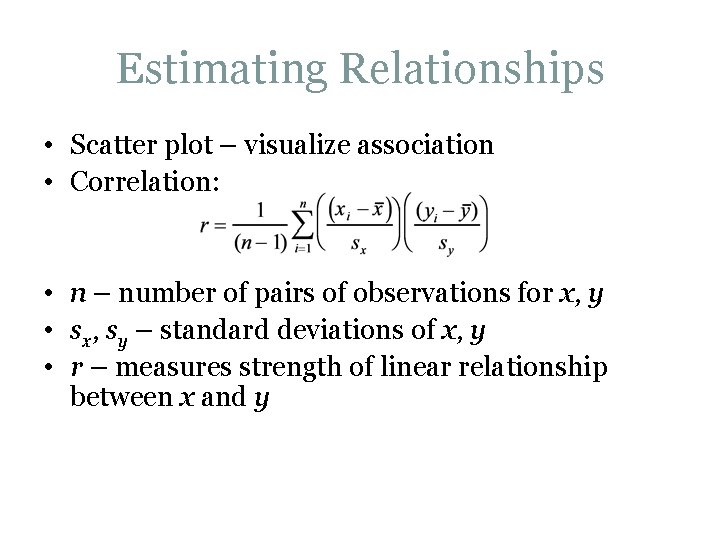
Estimating Relationships • Scatter plot – visualize association • Correlation: • n – number of pairs of observations for x, y • sx, sy – standard deviations of x, y • r – measures strength of linear relationship between x and y

r-statistic • • Independent of units of measurement Lies in range [-1, 1] r > 0 – positive association r < 0 – negative association r close to 1 (or – 1) implies a strong association r close to 0 implies a weak association Excel function: CORREL(xrange, yrange)

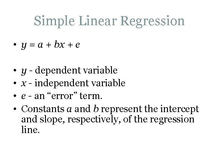
Simple Linear Regression • y = a + bx + e • • y - dependent variable x - independent variable e - an “error” term. Constants a and b represent the intercept and slope, respectively, of the regression line.

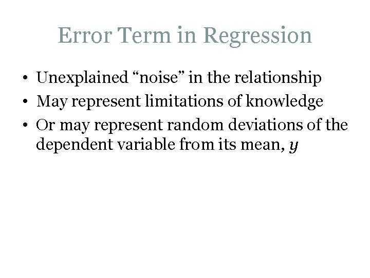
Error Term in Regression • Unexplained “noise” in the relationship • May represent limitations of knowledge • Or may represent random deviations of the dependent variable from its mean, y

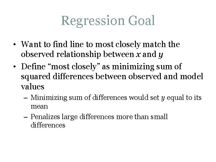
Regression Goal • Want to find line to most closely match the observed relationship between x and y • Define “most closely” as minimizing sum of squared differences between observed and model values – Minimizing sum of differences would set y equal to its mean – Penalizes large differences more than small differences

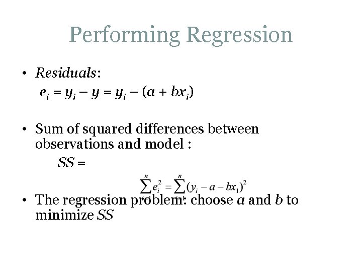
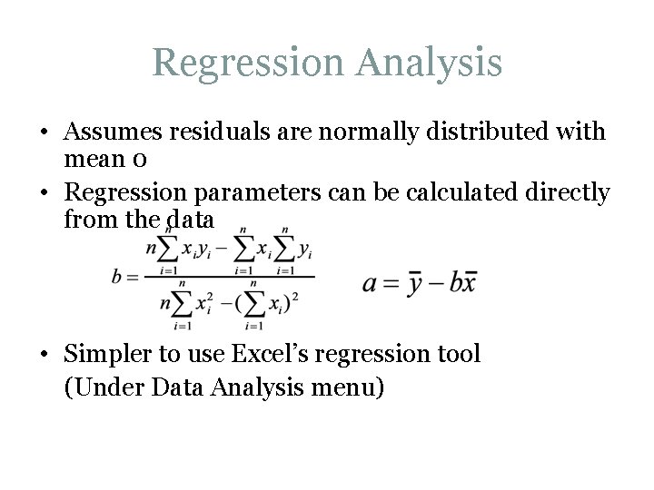
Performing Regression • Residuals: ei = yi – y = yi – (a + bxi) • Sum of squared differences between observations and model : SS = • The regression problem: choose a and b to minimize SS

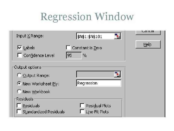
Regression Analysis • Assumes residuals are normally distributed with mean 0 • Regression parameters can be calculated directly from the data • Simpler to use Excel’s regression tool (Under Data Analysis menu)

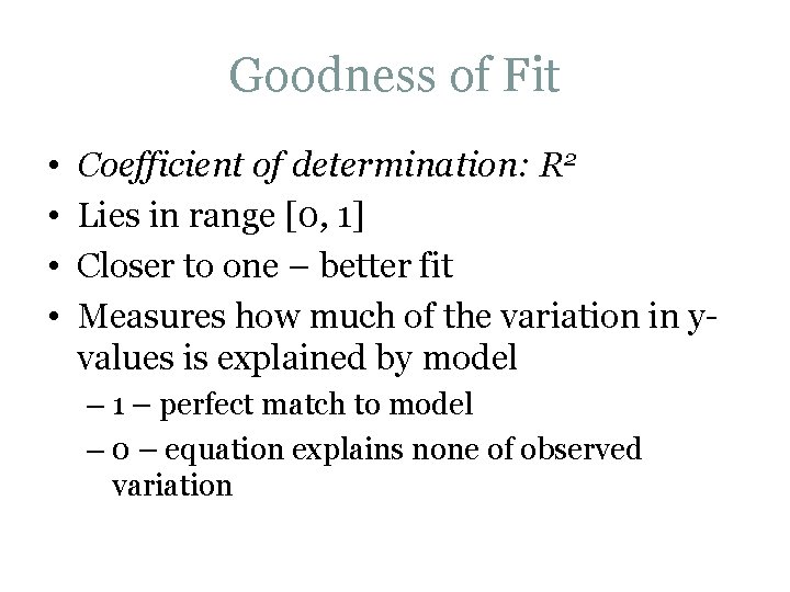
Goodness of Fit • • Coefficient of determination: R 2 Lies in range [0, 1] Closer to one – better fit Measures how much of the variation in yvalues is explained by model – 1 – perfect match to model – 0 – equation explains none of observed variation

Regression Window

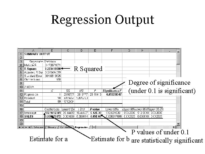
Regression Output R Squared Degree of significance (under 0. 1 is significant) Estimate for a P values of under 0. 1 Estimate for b are statistically significant

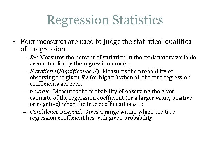
Regression Statistics • Four measures are used to judge the statistical qualities of a regression: – R 2: Measures the percent of variation in the explanatory variable accounted for by the regression model. – F-statistic (Significance F): Measures the probability of observing the given R 2 (or higher) when all the true regression coefficients are zero. – p-value: Measures the probability of observing the given estimate of the regression coefficient (or a larger value, positive or negative) when the true coefficient is zero. – Confidence interval: Gives a range within which the true regression coefficient lies with given probability.

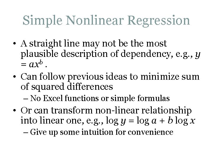
Simple Nonlinear Regression • A straight line may not be the most plausible description of dependency, e. g. , y = axb. • Can follow previous ideas to minimize sum of squared differences – No Excel functions or simple formulas • Or can transform non-linear relationship into linear one, e. g. , log y = log a + b log x – Give up some intuition for convenience

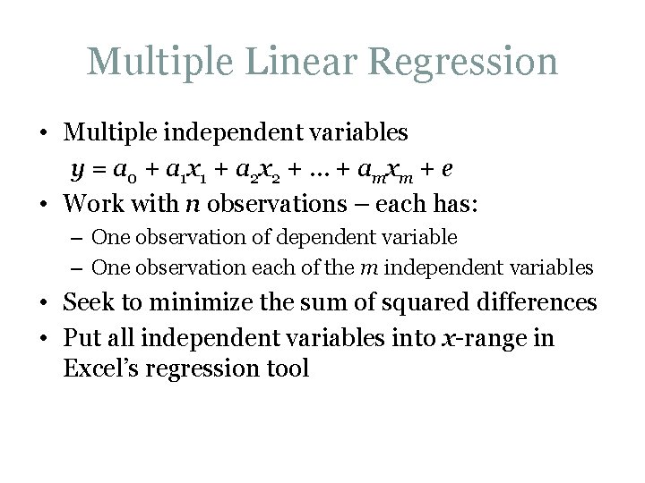
Multiple Linear Regression • Multiple independent variables y = a 0 + a 1 x 1 + a 2 x 2 + … + a mx m + e • Work with n observations – each has: – One observation of dependent variable – One observation each of the m independent variables • Seek to minimize the sum of squared differences • Put all independent variables into x-range in Excel’s regression tool

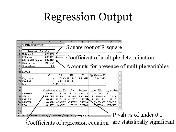
Regression Output Square root of R square Coefficient of multiple determination Accounts for presence of multiple variables P values of under 0. 1 Coefficients of regression equation are statistically significant

Values to Include in Regression • Ideally pick values that can be justified based on practical or theoretical grounds • Could choose set that generates largest value of adjusted R 2 • Also could choose based on those with significant p-values for coefficients • Remember that good models require good forecasts for the independent variables.

Regression Assumptions • Errors in the regression model: – Follow a Normal distribution – Are mutually independent – Have the same variance • Linearity is assumed to hold