PREDICTION AND REGRESSION REGRESSION Regression allows the researcher

PREDICTION AND REGRESSION

REGRESSION Regression allows the researcher to make predictions of the likely values of the dependent variable Y – from known values of independent variable X in a simple linear regression, – or from known values of a combination of independent variables D, E, and F in multiple linear regression.

Use of Regression We often need to determine such issues as: • the relationship between decrease in pollutant emissions and a factory’s annual expenditure on pollution abatement devices. If we spend more on abatement can we decrease emissions even more? • how investment varies with interest rates. Can we predict how much more investment occurs with a 1% interest rise? • how unemployment varies with inflation. What level will unemployment reach if inflation increases by 2% this year ?

Examples of simple and multiple linear regression questions • In simple linear regression – does the number of customers predict value of sales - variations in one IV predicting variations in one DV • In multiple linear regression – does maximizing value of sales depend on a particular combination of the number of customers, price variations, number of sales outlets, number of salespersons, etc

REGRESSION • Regression therefore investigates relationships between IV and DV in terms of the predictive ability of the IV to predict (estimate) the DV • It is therefore closely linked to correlation and shares many of the assumptions of ‘r’, e. g. – the relationships should be linear – the measurements of both the IV and DV variables must be interval or ratio (scale data)

IMPORTANT CONCEPTS • Predictor variable. – A variable (IV) from which a value is used to estimate a value on another variable (DV) • Criterion variable. – A variable (DV) a value of which is estimated from a value of the predictor variable (IV)

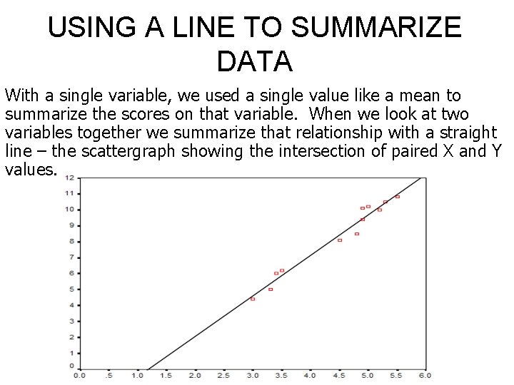
USING A LINE TO SUMMARIZE DATA With a single variable, we used a single value like a mean to summarize the scores on that variable. When we look at two variables together we summarize that relationship with a straight line – the scattergraph showing the intersection of paired X and Y values.

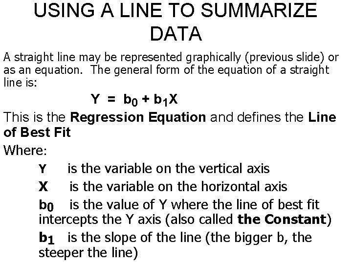
USING A LINE TO SUMMARIZE DATA A straight line may be represented graphically (previous slide) or as an equation. The general form of the equation of a straight line is: Y = b 0 + b 1 X This is the Regression Equation and defines the Line of Best Fit Where: Y is the variable on the vertical axis X is the variable on the horizontal axis b 0 is the value of Y where the line of best fit intercepts the Y axis (also called the Constant) b 1 is the slope of the line (the bigger b, the steeper the line)

LINE OF BEST FIT • This is the straight line on a scattergraph that ‘fits’ the scatter points best, i. e. as closely as possible • This line of best fit minimizes the deviations from the line of all the points on a scattergraph • It makes errors of prediction of Y as small as possible.

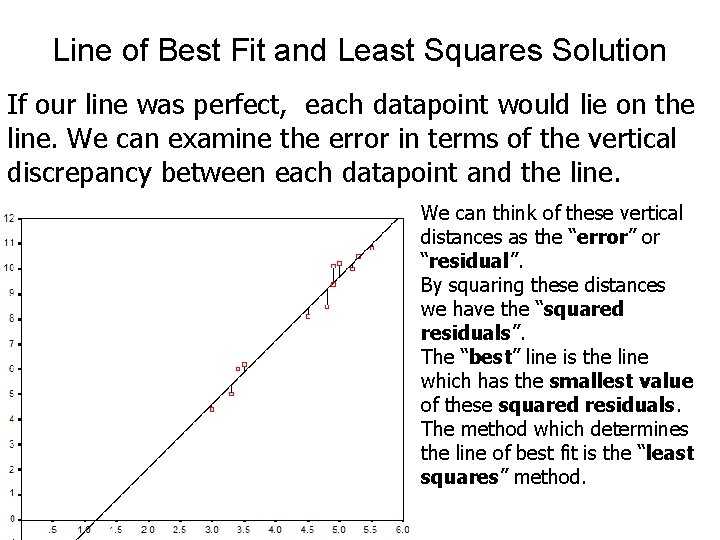
Line of Best Fit and Least Squares Solution If our line was perfect, each datapoint would lie on the line. We can examine the error in terms of the vertical discrepancy between each datapoint and the line. We can think of these vertical distances as the “error” or “residual”. By squaring these distances we have the “squared residuals”. The “best” line is the line which has the smallest value of these squared residuals. The method which determines the line of best fit is the “least squares” method.

The Least Squares Solution • This is the model that minimizes the sum of the squared deviations from each point to the regression line. • The regression line defined by the least squares model is the line of best fit.

HOW ACCURATE IS OUR ESTIMATE OF Y? • In reality a value of X may occur several times in a data set, but we could very well get a slightly different Y value each time. • Regression analysis assumes that this distribution of Y values is normally distributed. This distribution is centred at the mean of the Y values. • The best our regression model or SPSS can do is estimate the average value for Y for any given X value.

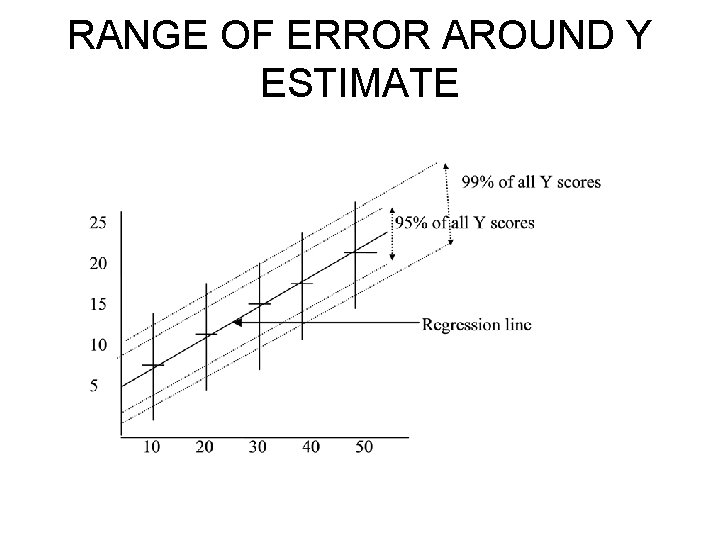
STANDARD ERROR OF THE ESTIMATE OF Y • Because Y is assumed to be normally distributed, it is possible to calculate a standard error for the estimated Y value which tells us how accurate our prediction is and what the range of error round it is. • The same confidence intervals (or significance levels) we have used before are employed. • E. g. The 95% confidence interval indicates the range of values within which the true value will fall 95% of the time.

RANGE OF ERROR AROUND Y ESTIMATE

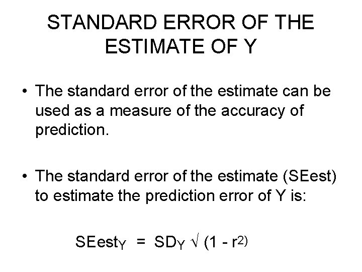
STANDARD ERROR OF THE ESTIMATE OF Y • The standard error of the estimate can be used as a measure of the accuracy of prediction. • The standard error of the estimate (SEest) to estimate the prediction error of Y is: SEest. Y = SDY (1 - r 2)

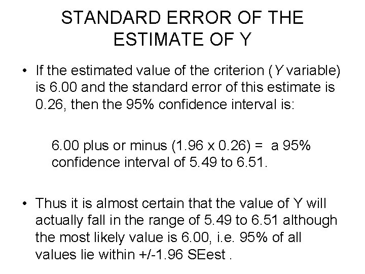
STANDARD ERROR OF THE ESTIMATE OF Y • If the estimated value of the criterion (Y variable) is 6. 00 and the standard error of this estimate is 0. 26, then the 95% confidence interval is: 6. 00 plus or minus (1. 96 x 0. 26) = a 95% confidence interval of 5. 49 to 6. 51. • Thus it is almost certain that the value of Y will actually fall in the range of 5. 49 to 6. 51 although the most likely value is 6. 00, i. e. 95% of all values lie within +/-1. 96 SEest.

ASSUMPTIONS OF REGRESSION • A minimum requirement is to have at least 15 times more cases than IV’s, i. e. with 3 IV’s - a minimum of 45 cases • Outliers should be removed. One extremely low or high value distorts the prediction by changing the angle of slope of the regression line • Differences between obtained and predicted DV values should be normally distributed and variance of residuals the same for all predicted scores (homoscedasticity)

ASSUMPTIONS OF REGRESSION • Regression procedures assume that the dispersion of points is linear • Prediction can only be made about a sample from the same population • Regression is less accurate where variance between variables differs • There is no implication that an increase in X causes an increase in Y. Simultaneous increase in X and Y may have been caused by an unknown third variable excluded from the study

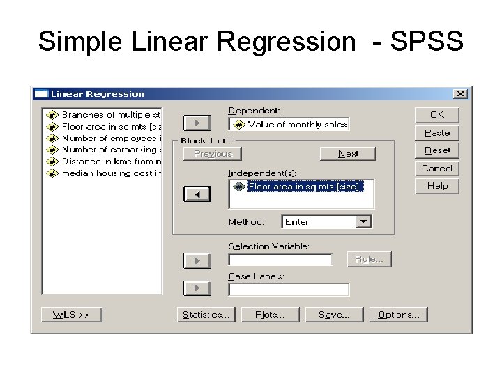
Simple Linear Regression - SPSS 1. Assume we want to predict ‘value of monthly sales’ from knowledge of ‘floor area in sq m. ’ 2. Select Analyse and then Regression. 3. Choose Linear to open the Linear Regression dialogue box 4. Click on the dependent variable (value of sales per month) and place it in the Dependent: box. 5. Select the independent variable (floor area in sq mts) and move it into Independent [s]: box 6. In Method box ensure Enter is selected.

Simple Linear Regression - SPSS

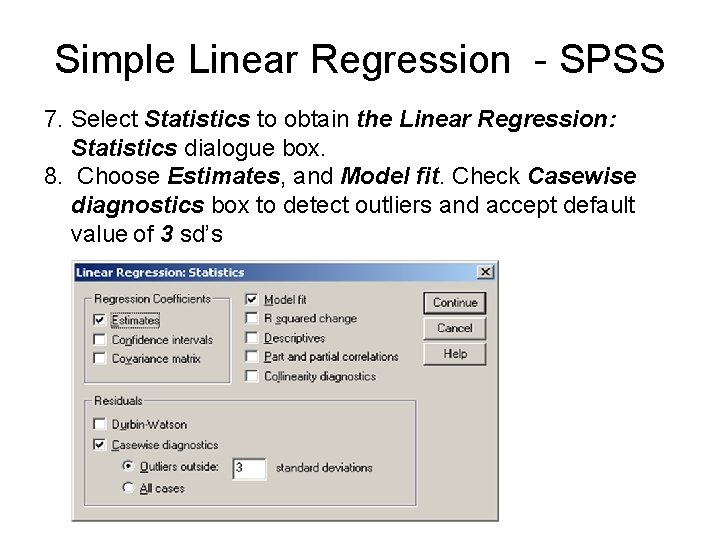
Simple Linear Regression - SPSS 7. Select Statistics to obtain the Linear Regression: Statistics dialogue box. 8. Choose Estimates, and Model fit. Check Casewise diagnostics box to detect outliers and accept default value of 3 sd’s

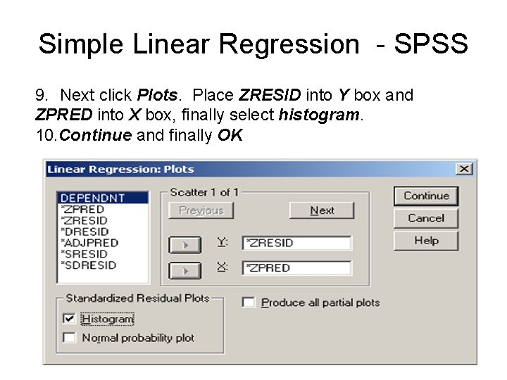
Simple Linear Regression - SPSS 9. Next click Plots. Place ZRESID into Y box and ZPRED into X box, finally select histogram. 10. Continue and finally OK

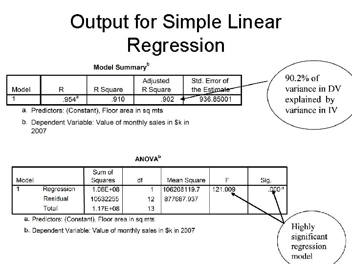
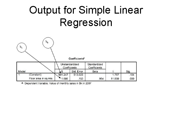
Output for Simple Linear Regression

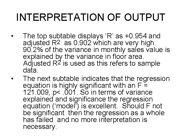
INTERPRETATION OF OUTPUT • • The top subtable displays ‘R’ as +0. 954 and adjusted R 2 as 0. 902 which are very high. 90. 2% of the variance in monthly sales value is explained by the variance in floor area. Adjusted R 2 is used as this refers to sample data. The next subtable indicates that the regression equation is highly significant with an F = 121. 009, p<. 001. So in terms of variance explained and significance the regression equation (‘model’) is excellent. Should F not be significant then the regression as a whole has failed and no more interpretation is necessary.

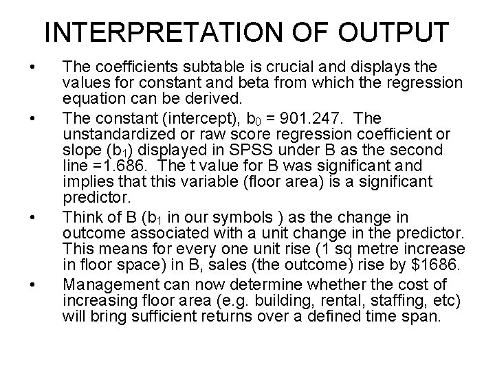
Output for Simple Linear Regression b 0 b 1

INTERPRETATION OF OUTPUT • • The coefficients subtable is crucial and displays the values for constant and beta from which the regression equation can be derived. The constant (intercept), b 0 = 901. 247. The unstandardized or raw score regression coefficient or slope (b 1) displayed in SPSS under B as the second line =1. 686. The t value for B was significant and implies that this variable (floor area) is a significant predictor. Think of B (b 1 in our symbols ) as the change in outcome associated with a unit change in the predictor. This means for every one unit rise (1 sq metre increase in floor space) in B, sales (the outcome) rise by $1686. Management can now determine whether the cost of increasing floor area (e. g. building, rental, staffing, etc) will bring sufficient returns over a defined time span.

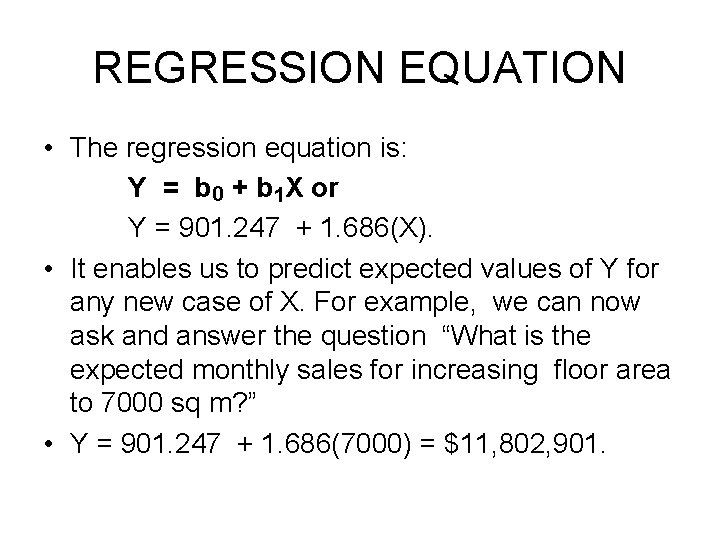
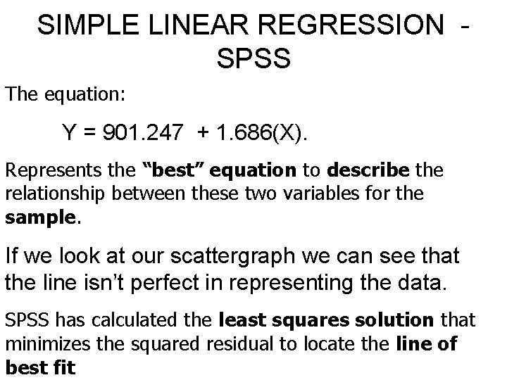
REGRESSION EQUATION • The regression equation is: Y = b 0 + b 1 X or Y = 901. 247 + 1. 686(X). • It enables us to predict expected values of Y for any new case of X. For example, we can now ask and answer the question “What is the expected monthly sales for increasing floor area to 7000 sq m? ” • Y = 901. 247 + 1. 686(7000) = $11, 802, 901.

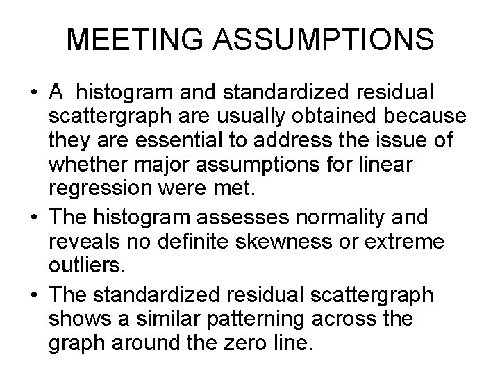
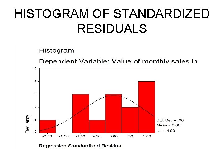
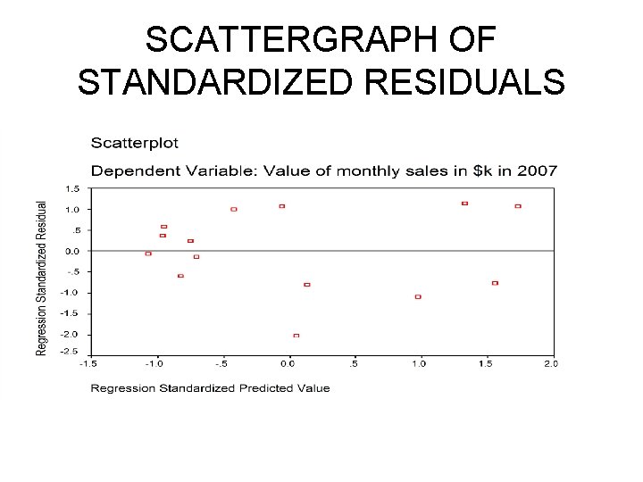
MEETING ASSUMPTIONS • A histogram and standardized residual scattergraph are usually obtained because they are essential to address the issue of whether major assumptions for linear regression were met. • The histogram assesses normality and reveals no definite skewness or extreme outliers. • The standardized residual scattergraph shows a similar patterning across the graph around the zero line.

HISTOGRAM OF STANDARDIZED RESIDUALS

SCATTERGRAPH OF STANDARDIZED RESIDUALS

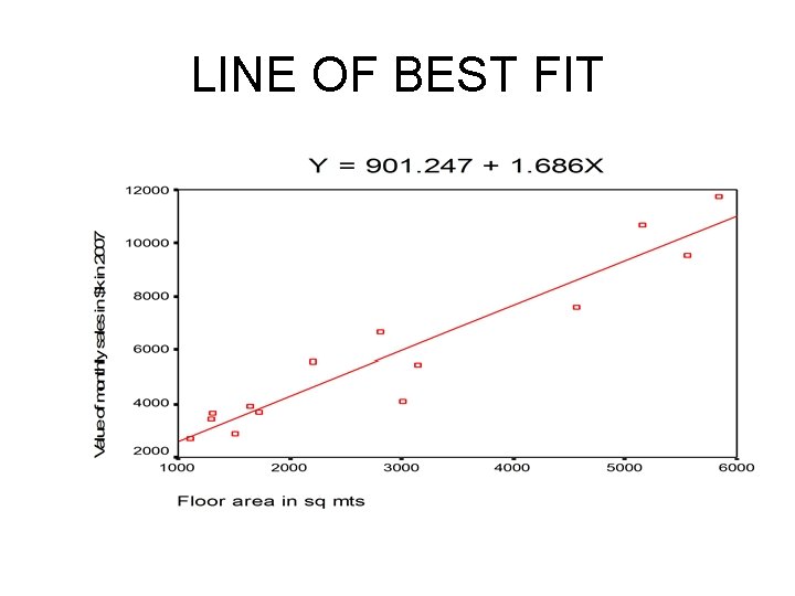
REGRESSION LINE ON SCATTERGRAPH • A scattergraph provides a clear visual presentation of what may seem to be mathematical diarrhoea – Select Graphs then Scatter. – Accept Simple option default, then select Define. – Move dependent variable (value of monthly sales) into the Y Axis: box. – Transfer the independent variable (floor area in sq mts) to the X Axis: box. – Select OK and the scattergraph will be displayed. • To draw the regression line on the displayed chart: – – Double click on the chart to select it for editing. In the Chart Dialogue box choose Chart and click on Options. Select Total in the Fit Line box. Select OK and the regression line is now displayed on the scattergraph

LINE OF BEST FIT

SIMPLE LINEAR REGRESSION SPSS The equation: Y = 901. 247 + 1. 686(X). Represents the “best” equation to describe the relationship between these two variables for the sample. If we look at our scattergraph we can see that the line isn’t perfect in representing the data. SPSS has calculated the least squares solution that minimizes the squared residual to locate the line of best fit

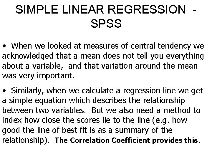
SIMPLE LINEAR REGRESSION SPSS • When we looked at measures of central tendency we acknowledged that a mean does not tell you everything about a variable, and that variation around the mean was very important. • Similarly, when we calculate a regression line we get a simple equation which describes the relationship between two variables. But we also need a method to index how close the scores lie to the line (e. g. how good the line of best fit is as a summary of the relationship). The Correlation Coefficient provides this.

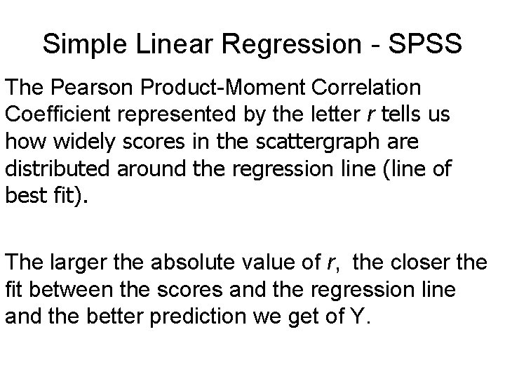
Simple Linear Regression - SPSS The Pearson Product-Moment Correlation Coefficient represented by the letter r tells us how widely scores in the scattergraph are distributed around the regression line (line of best fit). The larger the absolute value of r, the closer the fit between the scores and the regression line and the better prediction we get of Y.

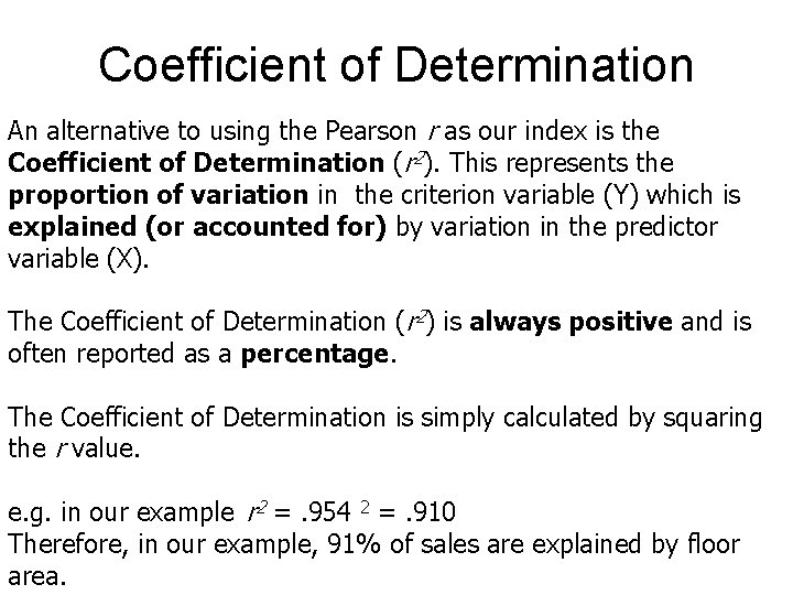
Coefficient of Determination An alternative to using the Pearson r as our index is the Coefficient of Determination (r 2). This represents the proportion of variation in the criterion variable (Y) which is explained (or accounted for) by variation in the predictor variable (X). The Coefficient of Determination (r 2) is always positive and is often reported as a percentage. The Coefficient of Determination is simply calculated by squaring the r value. e. g. in our example r 2 =. 954 2 =. 910 Therefore, in our example, 91% of sales are explained by floor area.

Coefficient of Determination • r 2 (simple linear regression) and R 2 (multiple regression), enable us to assess how well the line of best fit (the regression equation) fits the actual data. • It might be our line of best fit, but it could still lead to poor predictions. The higher the correlation (and by implication the coefficient of determination) the better the line fits the data as more variance is explained.

MULTIPLE REGRESSION • Multiple Regression – a technique for estimating the value of the criterion variable (Y) from values on two or more other predictor variables (X’s) • Multiple Correlation (R) – a measure of the correlation of one dependent variable with a combination of two or more predictor variables. – Coefficient of Multiple Determination is R 2

MULTIPLE REGRESSION • So far we have focused on simple linear regression in which one independent or predictor variable was used to predict the value of a dependent or criterion variable. • But there can be many other potential predictors that might establish a better or more meaningful prediction. With more than one predictor variable we use multiple regression. • E. g. the prediction of individual income may depend on a combination of education, job experience, gender, age, etc

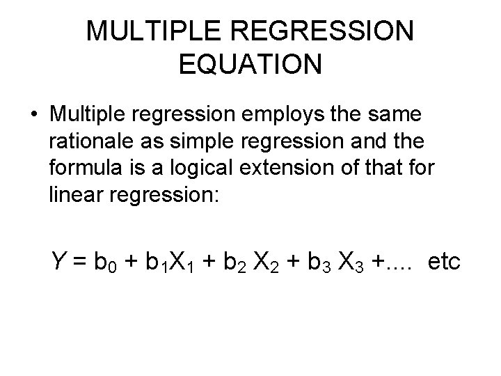
MULTIPLE REGRESSION EQUATION • Multiple regression employs the same rationale as simple regression and the formula is a logical extension of that for linear regression: Y = b 0 + b 1 X 1 + b 2 X 2 + b 3 X 3 +. . etc

Assumptions of Multiple Regression • In addition to the assumptions noted for simple linear regression, one further major assumption applies in multiple regression. Very high correlations between IV’s should be avoided. • This is multicollinearity. Create a correlation matrix and inspect for high correlations of 0. 90 and above as this implies the two variables are measuring the same variance and will overinflate R. Therefore only one of the two variables is needed. • The Variance Inflation Factor (VIF) measures the degree to which collinearity among the predictors degrades the precision of an estimate. Typically a VIF value greater than 10. 0 is of concern.

TYPES OF MULTIPLE REGRESSION There are three types of Multiple Regression 1. Standard Multiple regression 2. Hierarchical Multiple Regression 3. Stepwise Multiple Regression

STANDARD MULTIPLE REGRESSION The SPSS procedure is the same as that for simple linear regression except that two or more predictor variables are entered.

Hierarchical Multiple Regression • While standard multiple regression considers all the predictors at once, hierarchical multiple regression is used when researchers are interested in looking at the influence of several predictor variables in a sequential way. • That is, they want to know what the prediction will be for the first predictor variable, and then how much is added to the overall prediction by including a second predictor variable, and then perhaps how much more is added by including a third predictor variable, and so on.

HIERARCHICAL MULTIPLE REGRESSION The researcher determines the order of entry of the IV’s or predictors into the equation based on theoretical knowledge The amount that each successive variable adds to the overall prediction is described in terms of an increase in R 2, the proportion of variance accounted for or explained.

Hierarchical Multiple Regression • To enter the predictor variables: – Select the first independent variable and move it into Independent [s]: box Block 1 of 1 – Click Next and select the second independent variable and move it into Independent [s]: box Block 2 of 2 – Click Next and select the third independent variable and move it into Independent [s]: box Block 3 of 3. Continue with this process until all IV’s are entered.

STEPWISE MULTIPLE REGRESSION Decisions about the order of entry for predictors are made solely on statistical decision in the stepwise regression SPSS programme. – Forward entry involves the entry of the IV’s one at a time as selected by SPSS – Backward selection is the reverse of the forward entry commencing with the insertion of all IV’s with SPSS deleting successively those that fail to meet certain critical significance values. – SPSS allows you to choose either forward or backward entry by clicking on the Method box