Regression Artificial Neural Networks 07032017 Regression Regression Supervised

Regression, Artificial Neural Networks 07/03/2017

Regression

Regression – Supervised learning: Based on training examples, learn a modell which works fine on previously unseen examples. – Regression: forecasting real values

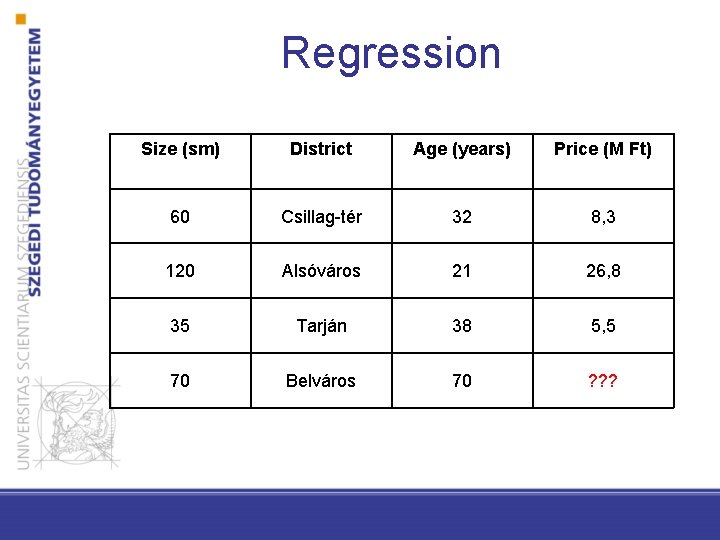
Regression Size (sm) District Age (years) Price (M Ft) 60 Csillag-tér 32 8, 3 120 Alsóváros 21 26, 8 35 Tarján 38 5, 5 70 Belváros 70 ? ? ?

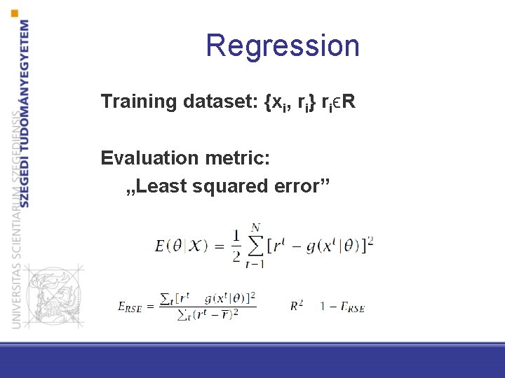
Regression Training dataset: {xi, ri} riϵR Evaluation metric: „Least squared error”

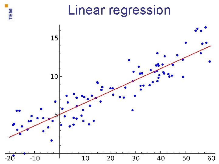
Linear regression

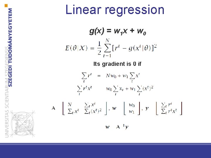
Linear regression g(x) = w 1 x + w 0 Its gradient is 0 if

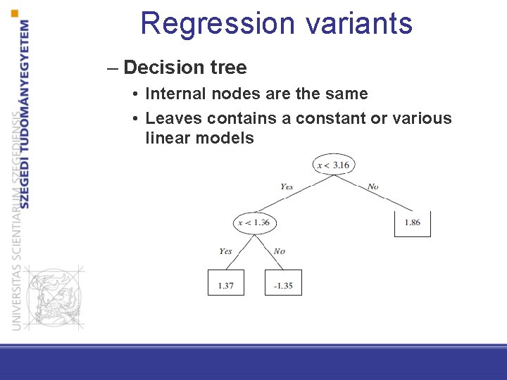
Regression variants – Decision tree • Internal nodes are the same • Leaves contains a constant or various linear models

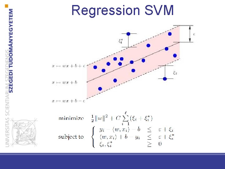
Regression SVM

Artificial Neural Networks

Artificial neural networks • Motivation: the simulation of the neuo system (human brain)’s information processing mechanisms • Structure: huge amount of densely connected, mutally operating processing units (neurons) • It learns from experiences (training instances)

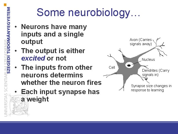
Some neurobiology… • Neurons have many inputs and a single output • The output is either excited or not • The inputs from other neurons determins whether the neuron fires • Each input synapse has a weight

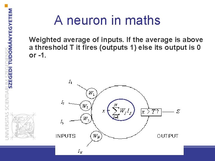
A neuron in maths Weighted average of inputs. If the average is above a threshold T it fires (outputs 1) else its output is 0 or -1.

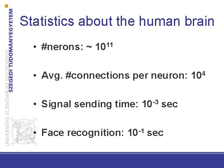
Statistics about the human brain • #nerons: ~ 1011 • Avg. #connections per neuron: 104 • Signal sending time: 10 -3 sec • Face recognition: 10 -1 sec

Motivation (machine learning point of view) • Goal: non-linear classification – Linear machines are not satisfactory at several real world situations – Which non-linear function family to choose? – Neural networks: latent non-linear patterns will be machine learnt

Perceptron

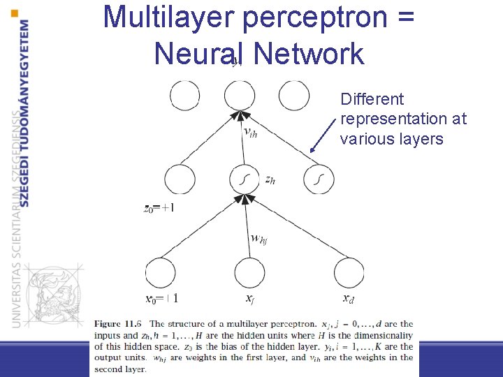
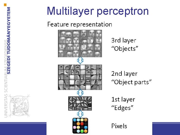
Multilayer perceptron = Neural Network Different representation at various layers

Multilayer perceptron

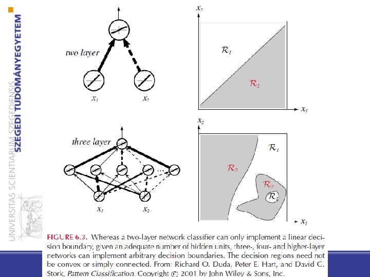
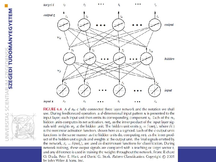
Feedforward neural networks • Connection only to the next layer • The weights of the connections (between two layers) can be changed • Activation functions are used to calculate whether the neuron fires • Three-layer network: • Input layer • Hidden layer • Output layer

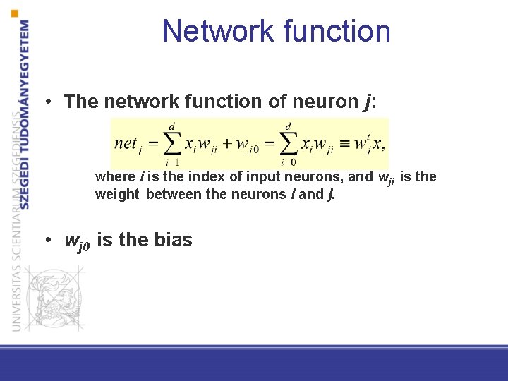
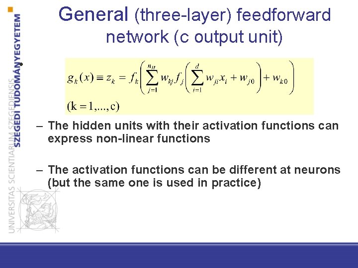
Network function • The network function of neuron j: where i is the index of input neurons, and wji is the weight between the neurons i and j. • wj 0 is the bias

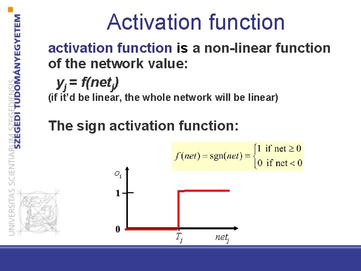
Activation function activation function is a non-linear function of the network value: yj = f(netj) (if it’d be linear, the whole network will be linear) The sign activation function: oi 1 0 Tj netj

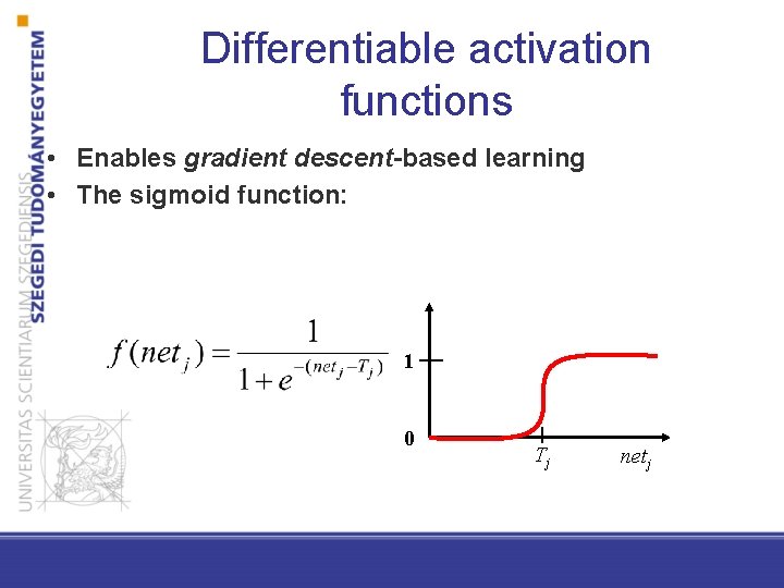
Differentiable activation functions • Enables gradient descent-based learning • The sigmoid function: 1 0 Tj netj

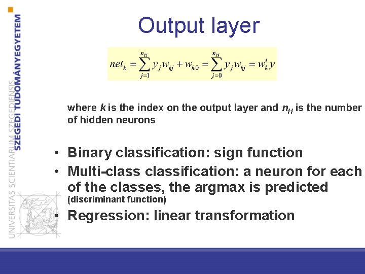
Output layer where k is the index on the output layer and n. H is the number of hidden neurons • Binary classification: sign function • Multi-classification: a neuron for each of the classes, the argmax is predicted (discriminant function) • Regression: linear transformation

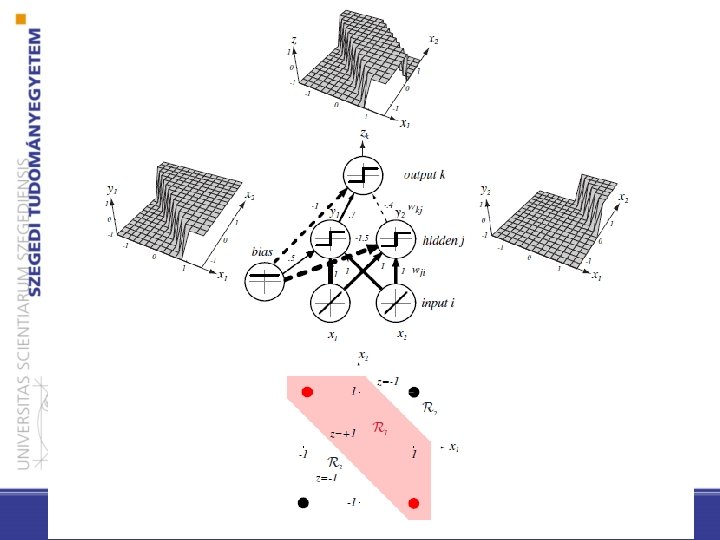
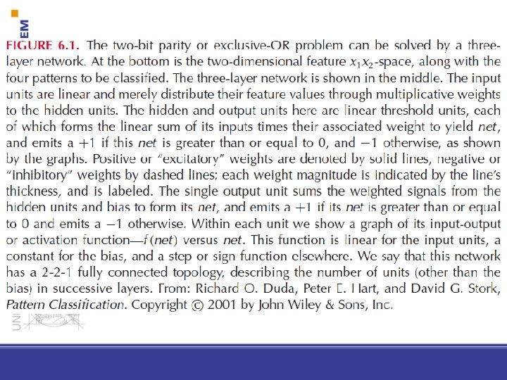
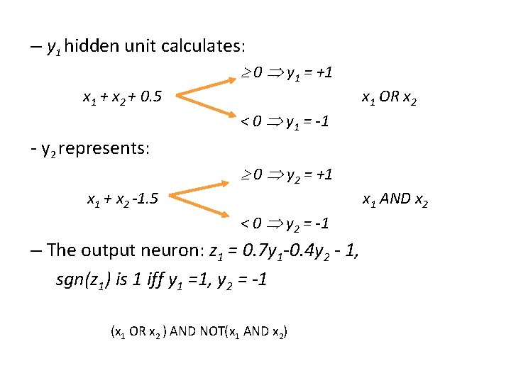
– y 1 hidden unit calculates: 0 y 1 = +1 x 1 + x 2 + 0. 5 - y 2 represents: x 1 + x 2 -1. 5 < 0 y 1 = -1 x 1 OR x 2 0 y 2 = +1 < 0 y 2 = -1 – The output neuron: z 1 = 0. 7 y 1 -0. 4 y 2 - 1, sgn(z 1) is 1 iff y 1 =1, y 2 = -1 (x 1 OR x 2 ) AND NOT(x 1 AND x 2) x 1 AND x 2

General (three-layer) feedforward network (c output unit) • – The hidden units with their activation functions can express non-linear functions – The activation functions can be different at neurons (but the same one is used in practice)

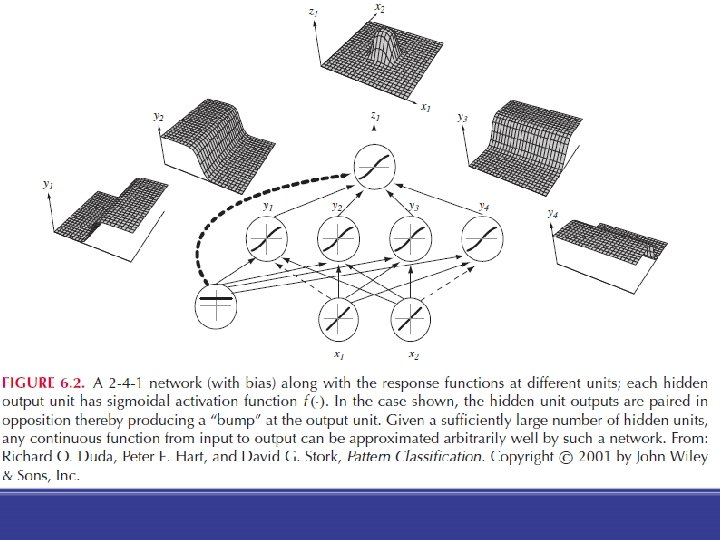
Universal approximation theorem states that a feed-forward network with a single hidden layer containing a finite number of neurons can approximate any continuous functions But theorem does not give any hint on who to design activation functions for problems/datasets

Training of neural networks (backpropagation)

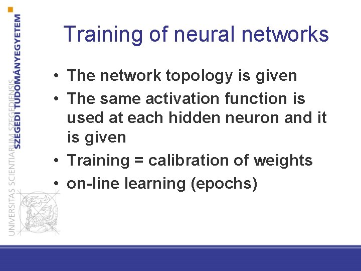
Training of neural networks • The network topology is given • The same activation function is used at each hidden neuron and it is given • Training = calibration of weights • on-line learning (epochs)

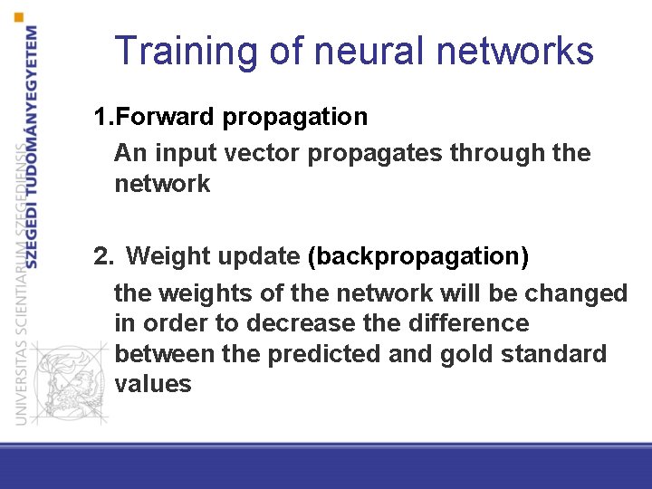
Training of neural networks 1. Forward propagation An input vector propagates through the network 2. Weight update (backpropagation) the weights of the network will be changed in order to decrease the difference between the predicted and gold standard values

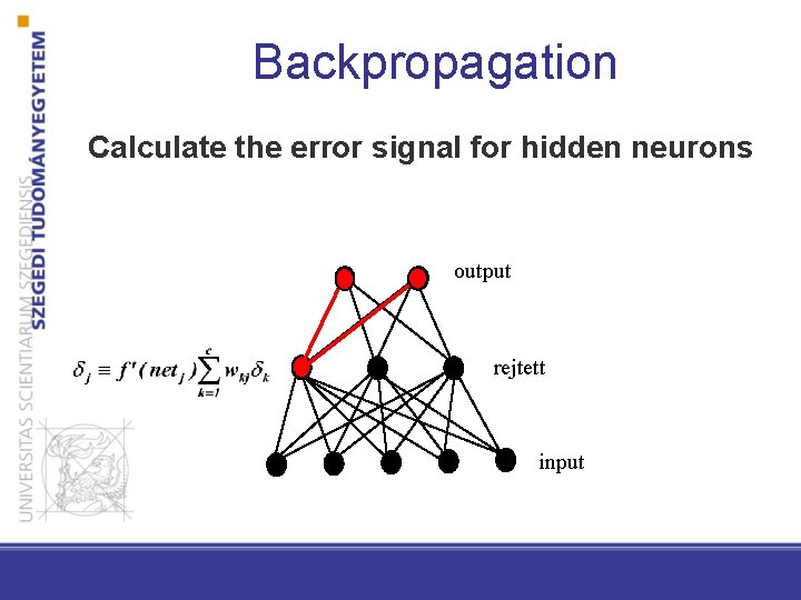
Training of neural networks we can calculate (propagate back) the error signal for each hidden neuron

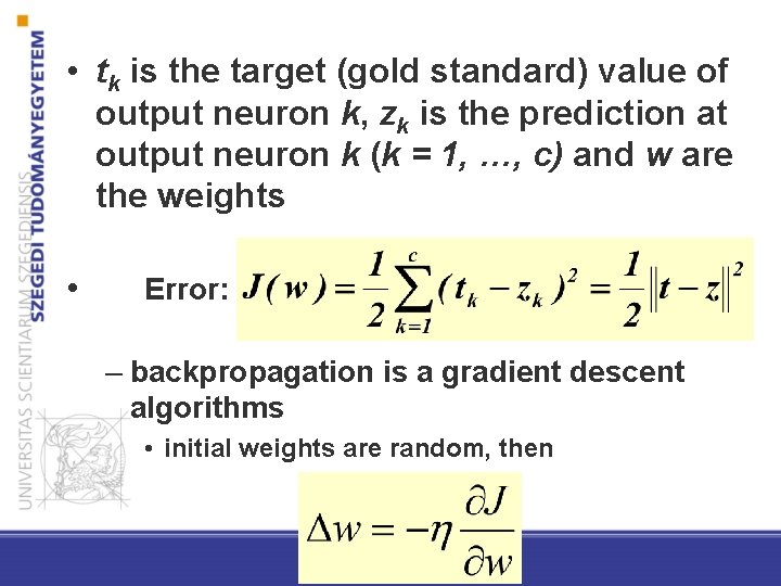
• tk is the target (gold standard) value of output neuron k, zk is the prediction at output neuron k (k = 1, …, c) and w are the weights • Error: – backpropagation is a gradient descent algorithms • initial weights are random, then

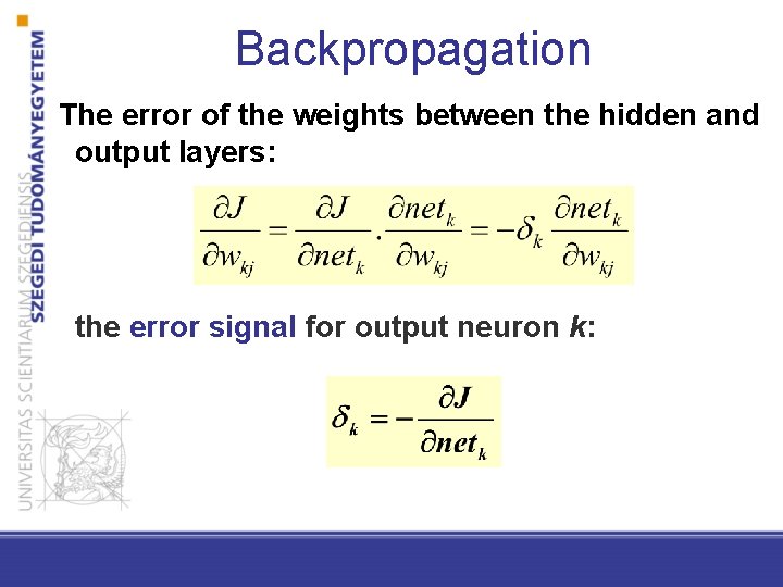
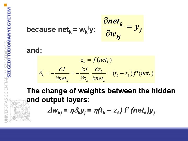
Backpropagation The error of the weights between the hidden and output layers: the error signal for output neuron k:

because netk = wkty: and: The change of weights between the hidden and output layers: wkj = kyj = (tk – zk) f’ (netk)yj

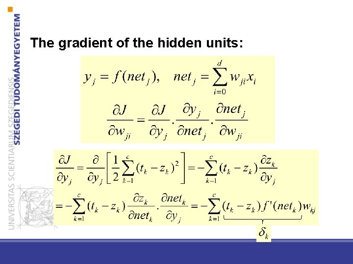
The gradient of the hidden units:

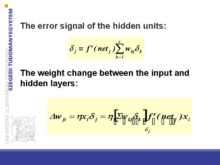
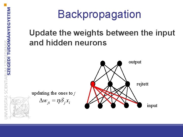
The error signal of the hidden units: The weight change between the input and hidden layers:

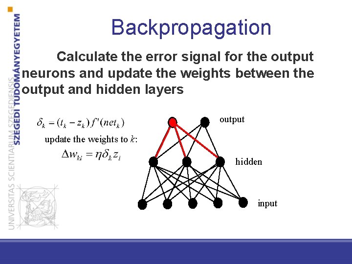
Backpropagation Calculate the error signal for the output neurons and update the weights between the output and hidden layers output update the weights to k: hidden input

Backpropagation Calculate the error signal for hidden neurons output rejtett input

Backpropagation Update the weights between the input and hidden neurons output rejtett updating the ones to j input

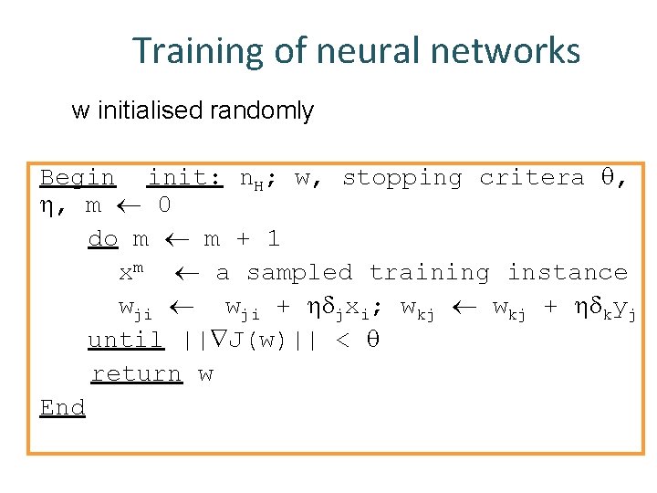
Training of neural networks w initialised randomly Begin init: n. H; w, stopping critera , , m 0 do m m + 1 xm a sampled training instance wji + jxi; wkj + kyj until || J(w)|| < return w End

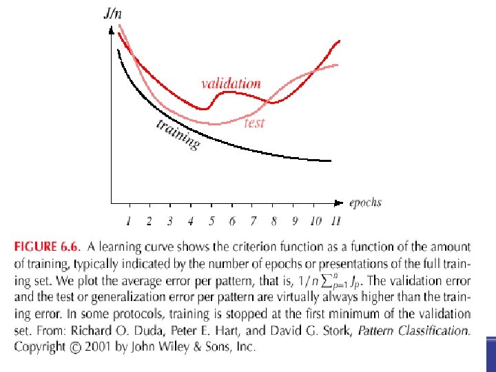
Stopping based on the performance on a validation dataset – The usage of unseen training instances for estimating the performance of supervised learning (to avoid overfitting) – Stopping at the minimum error on the validation set

Notes on backpropagation • it can be stack at local minima • In practice, the local minima is close to the global one • Multiple training starting from various randomly initalized weights might help – we can take the trained network with the minimal error (on a validation set) – there are voting schema for voting the networks

Questions of network design • How many hidden neurons? – few neurons cannot learn complex patterns – too many neurons can easily overfit – validation set? • Learning rate!?

Deep learning

History of neural networks • Perceptron: one of the first machine learners ~1950 • Backpropagation: multilayer perceptrons, 1975 • Deep learning: popular again 2006 -

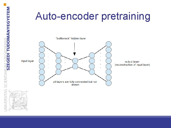
Auto-encoder pretraining

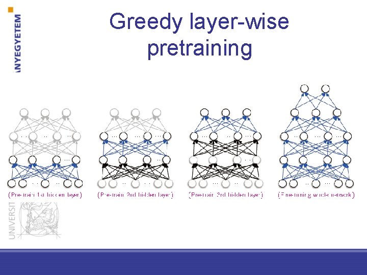
Greedy layer-wise pretraining

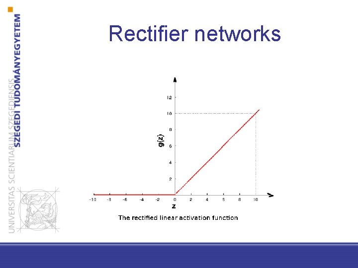
Rectifier networks

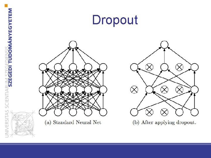
Dropout

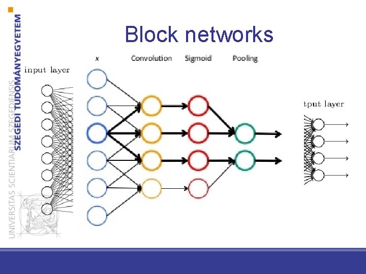
Block networks

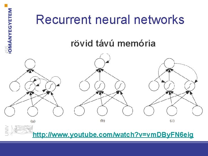
Recurrent neural networks rövid távú memória http: //www. youtube. com/watch? v=vm. DBy. FN 6 eig