Topic 3 Regression Correlation Analysis correlation analysis expresses

Topic 3: Regression

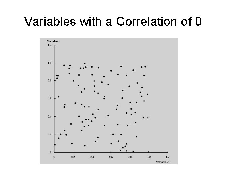
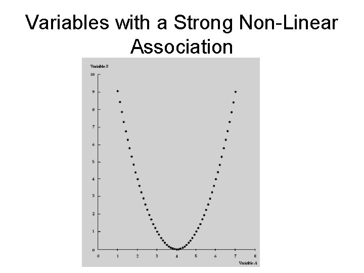
Correlation Analysis • correlation analysis expresses the relationship between two data series using a single number. • The correlation coefficient is a measure of how closely related two data series are. • The correlation coefficient measures the linear association between two variables.

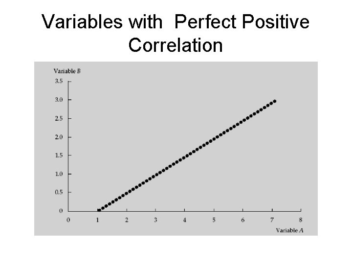
Variables with Perfect Positive Correlation

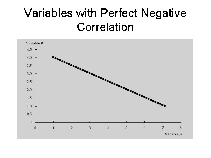
Variables with Perfect Negative Correlation

Variables with a Correlation of 0

Variables with a Strong Non-Linear Association

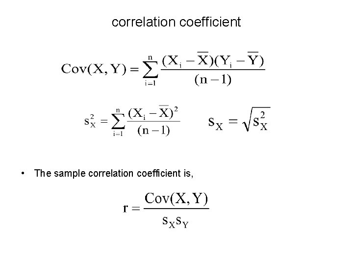
correlation coefficient • The sample correlation coefficient is,

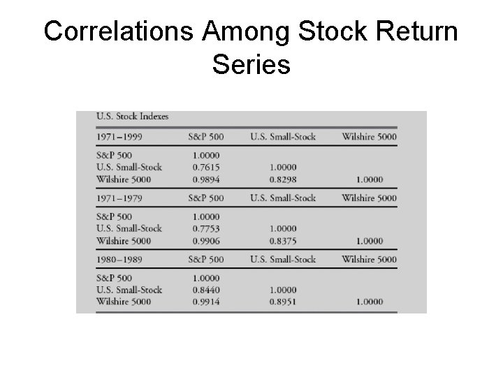
Correlations Among Stock Return Series

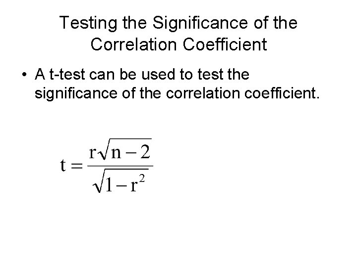
Testing the Significance of the Correlation Coefficient • A t-test can be used to test the significance of the correlation coefficient.

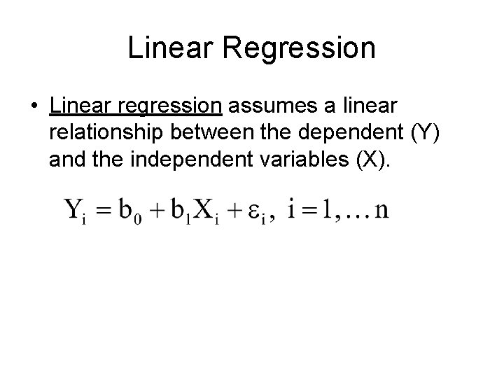
Linear Regression • Linear regression assumes a linear relationship between the dependent (Y) and the independent variables (X).

Assumptions of the Linear Regression Model • The relationship between the dependent variable, Y, and the independent variable, X is linear in the parameters b 0 and b 1. • The independent variable, X , is not random. • The expected value of the error term is 0. • The variance of the error term is the same for all observations. • The error term, ε, is uncorrelated across observations. • The error term, ε, is normally distributed.

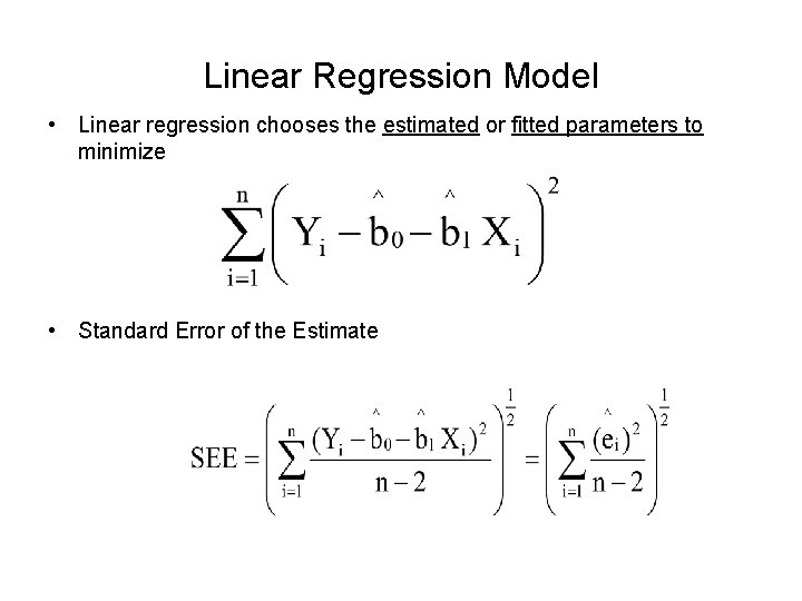
Linear Regression Model • Linear regression chooses the estimated or fitted parameters to minimize • Standard Error of the Estimate

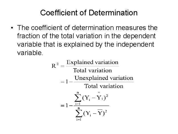
Coefficient of Determination • The coefficient of determination measures the fraction of the total variation in the dependent variable that is explained by the independent variable.

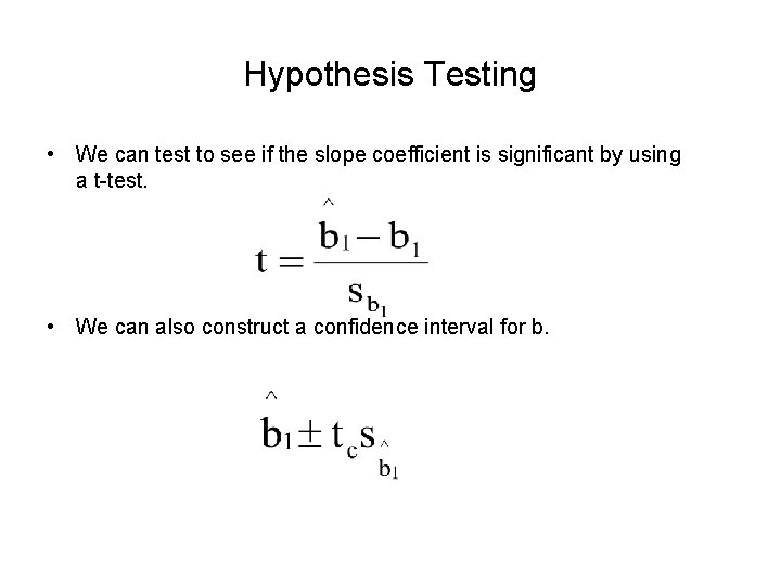
Hypothesis Testing • We can test to see if the slope coefficient is significant by using a t-test. • We can also construct a confidence interval for b.

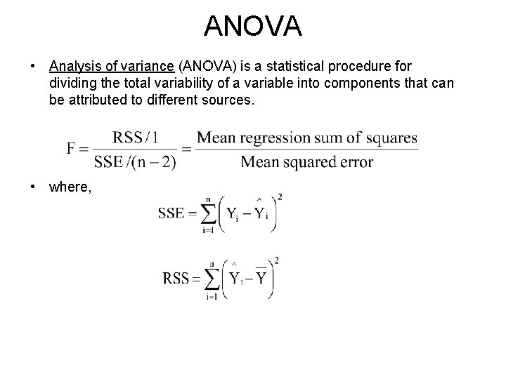
ANOVA • Analysis of variance (ANOVA) is a statistical procedure for dividing the total variability of a variable into components that can be attributed to different sources. • where,

Limitations of Regression Analysis • Regression relations can change over time, known as the issue of parameter instability. • Use of regression results specific to investment contexts is that public knowledge of regression relationships may negate their future usefulness. • If the regression assumptions are violated, hypothesis tests and predictions based on linear regression will not be valid.

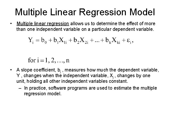
Multiple Linear Regression Model • Multiple linear regression allows us to determine the effect of more than one independent variable on a particular dependent variable. • A slope coefficient, bj , measures how much the dependent variable, Y , changes when the independent variable, Xj , changes by one unit, holding all other independent variables constant. – In practice, software programs are used to estimate the multiple regression model.

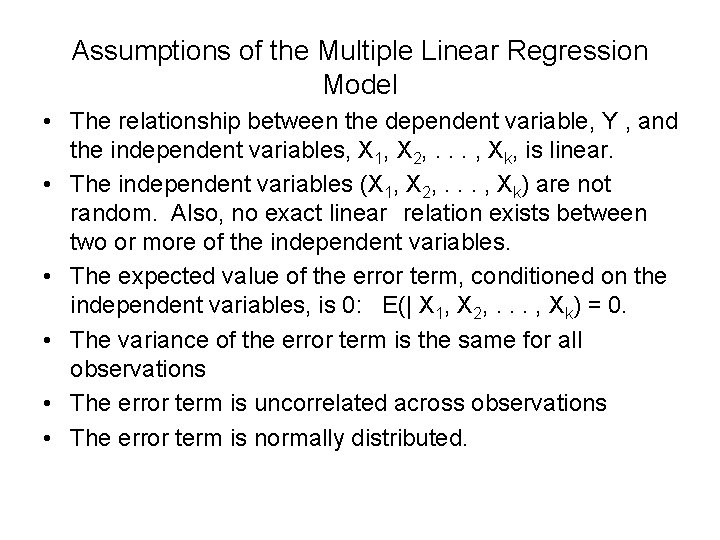
Assumptions of the Multiple Linear Regression Model • The relationship between the dependent variable, Y , and the independent variables, X 1, X 2, . . . , Xk, is linear. • The independent variables (X 1, X 2, . . . , Xk) are not random. Also, no exact linear relation exists between two or more of the independent variables. • The expected value of the error term, conditioned on the independent variables, is 0: E(| X 1, X 2, . . . , Xk) = 0. • The variance of the error term is the same for all observations • The error term is uncorrelated across observations • The error term is normally distributed.

Testing Whether All Population Regression Coefficients Equal 0 • We illustrated how to conduct hypothesis tests on regression coefficients individually using a t-test. • But what about the significance of the regression as a whole? – We test the null hypothesis that all the slope coefficients in a regression are simultaneously equal to 0 by using an F-test.

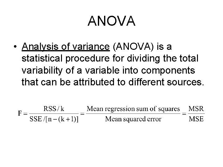
ANOVA • Analysis of variance (ANOVA) is a statistical procedure for dividing the total variability of a variable into components that can be attributed to different sources.

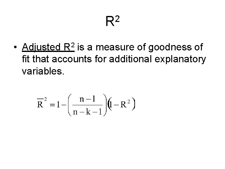
R 2 • Adjusted R 2 is a measure of goodness of fit that accounts for additional explanatory variables.

Using Dummy Variables • A dummy variable is qualitative variable that takes on a value of 1 if a particular condition is true and 0 if that condition is false. – used to account for qualitative variables such male or female, month of the year effects, etc.

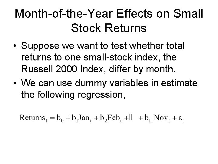
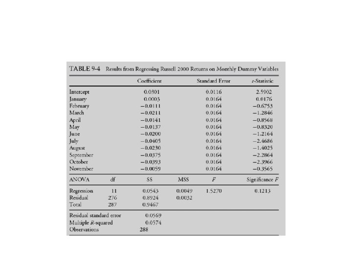
Month-of-the-Year Effects on Small Stock Returns • Suppose we want to test whether total returns to one small-stock index, the Russell 2000 Index, differ by month. • We can use dummy variables in estimate the following regression,

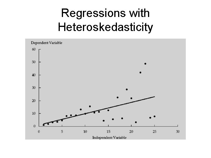
Violations of Regression Assumptions • Inference based on an estimated regression model rests on certain assumptions being met. • Violations may cause the inferences made to be invalid. • Heteroskedasticity occurs when the variance of the errors differs across observations. – does not affect consistency – causes the F-test for the overall significance to be unreliable. – t-tests for the significance of individual regression coefficients are unreliable because heteroskedasticity introduces bias into estimators of the standard error of regression coefficients.

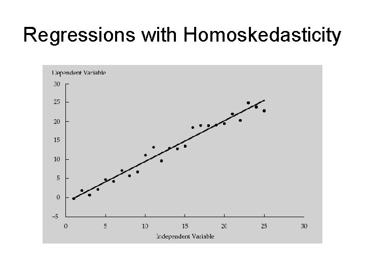
Regressions with Homoskedasticity

Regressions with Heteroskedasticity

Testing for Heteroskedasticity • The Breusch–Pagan test consists of regressing the squared residuals from the estimated regression equation on the independent variables in the regression. – If no conditional heteroskedasticity exists, the independent variables will not explain much of the variation in the squared residuals. – If conditional heteroskedasticity is present in the original regression, however, the independent variables will explain a significant portion of the variation in the squared residuals.

Correcting for Heteroskedasticity • Two different methods to correct the effects of conditional heteroskedasticity: – computing robust standard errors, corrects the standard errors of the linear regression model’s estimated coefficients to account for the conditional heteroskedasticity. – Generalized least squares, modifies the original equation in an attempt to eliminate the heteroskedasticity.

Serial Correlation • When regression errors are correlated across observations, we say that they are serially correlated (or autocorrelated). – Serial correlation most typically arises in time-series regressions. – The principal problem caused by serial correlation in a linear regression is an incorrect estimate of the regression coefficient standard errors • Positive serial correlation is serial correlation in which a positive error for one observation increases the chance of a positive error for another observation.

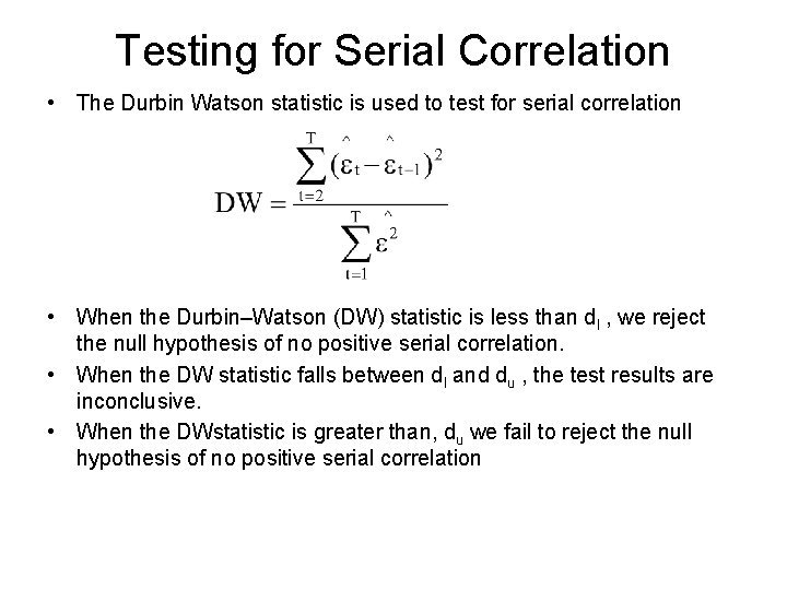
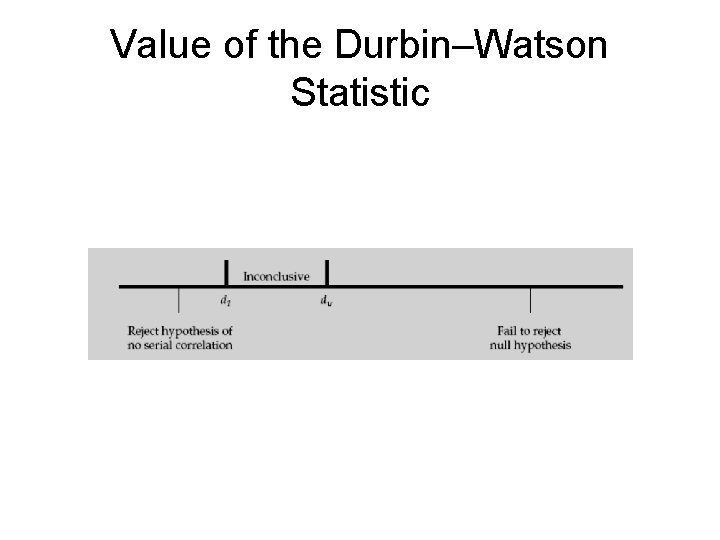
Testing for Serial Correlation • The Durbin Watson statistic is used to test for serial correlation • When the Durbin–Watson (DW) statistic is less than dl , we reject the null hypothesis of no positive serial correlation. • When the DW statistic falls between dl and du , the test results are inconclusive. • When the DWstatistic is greater than, du we fail to reject the null hypothesis of no positive serial correlation

Value of the Durbin–Watson Statistic

Correcting for Serial Correlation • Two alternative remedial steps whena regression has significant serial correlation: – adjust the coefficient standard errors for the linear regression parameter estimates to account for the serial correlation. – modify the regression equation itself to eliminate the serial correlation.

Multicollinearity • Multicollinearity occurs when two or more independent variables (or combinations of independent variables) are highly (but not perfectly) correlated with each other. – does not affect the consistency of the OLS estimates of the regression coefficients – estimates become extremely imprecise and unreliable • The classic symptom of multicollinearity is a high R 2 (and significant F-statistic) even though the t-statistics on the estimated slope coefficients are not significant. • The most direct solution to multicollinearity is excluding one or more of the regression variables.

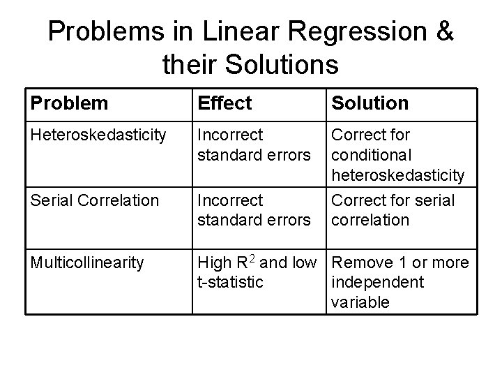
Problems in Linear Regression & their Solutions Problem Effect Solution Heteroskedasticity Incorrect standard errors Correct for conditional heteroskedasticity Serial Correlation Incorrect standard errors Correct for serial correlation Multicollinearity High R 2 and low Remove 1 or more t-statistic independent variable

Model Specification • Model specification refers to the set of variables included in the regression and the regression equation’s functional form. • Possible mispecifications include: – One or more important variables could be omitted from regression. – One or more of the regression variables may need to be transformed (for example, by taking the natural logarithm of the variable) before estimating the regression. – The regression model pools data from different samples that should not be pooled.

Models with Qualitative Dependent Variables • Qualitative dependent variables are dummy variables used as dependent variables instead of as independent variables. • The probit model, which is based on the normal distribution, estimates the probability that Y = 1 (a condition is fulfilled) given the value of the independent variable X. • The logit model is identical, except that it is based on the logistic distribution rather than the normal distribution. • Discriminant analysis yields a linear function, similar to a regression equation, which can then be used to create an overall score. Based on the score, an observation can be classified into categories such as bankrupt or not bankrupt.