INFS 815 QUANTITATIVE RESEARCH METHODS 1 MULTIPLE REGRESSION

INFS 815: QUANTITATIVE RESEARCH METHODS 1 MULTIPLE REGRESSION ANALYSIS (BASED ON MULTIVARIATE STATISTICS BY HAIR ET AL. , CHAPTER 4)

Learning Objectives 2 Upon completing this chapter, you should be able to do the following: 1. 2. 3. 4. 5. 6. Determine when regression analysis is the appropriate statistical tool in analyzing a problem. Understand how regression helps us make predictions using the least squares concept. Use dummy variables with an understanding of their interpretation. Be aware of the assumptions underlying regression analysis and how to assess them. Select an estimation technique and explain the difference between stepwise and simultaneous regression. Interpret the results of regression.

3 What is multiple regression analysis? Multiple regression analysis is the most widely-used dependence technique, with applications across all types of problems and all disciplines. Multiple regression is a statistical technique that can be used to analyze the relationship between a single dependent (criterion) variable and several independent (predictor) variables. The set of weighted independent variables forms the regression variate (also called as the regression equation or regression model), a linear combination of the independent variables that best predicts the dependent variable. In a nutshell, to apply multiple regression analysis: (a) the data must be metric or appropriately transformed, and (b) before deriving the regression equation, the researcher must decide upon which variable is to be dependent and which remaining variables will be independent. The regression variate is computed by a statistical procedure called ordinary least squares which minimizes the sum of squared prediction errors (residuals) in the equation. Multiple regression analysis has two possible objectives: 1. Prediction – attempts to predict a change in the dependent variable resulting from changes in multiple independent variables. 2. Explanation – enables the researcher to explain the variate by assessing the relative contribution of each independent variable to the regression equation.

Why do we use multiple regression analysis? 4 Multiple regression analysis is the technique of choice when the research objective is to predict a statistical relationship or to explain underlying relationships among variables. We also use multiple regression analysis because it enables the researcher to utilize two or more metric independent (predictor) variables in order to estimate the dependent (criterion) variable.

When do you use multiple regression analysis? 5 Multiple regression may be used any time the researcher has theoretical or conceptual justification for predicting or explaining the dependent variable with the set of independent variables. Multiple regression analysis is applicable in almost any business decision-making context as well. Common applications include models of: business forecasting firm performance consumer decision-making or preferences consumer attitudes new products quality control

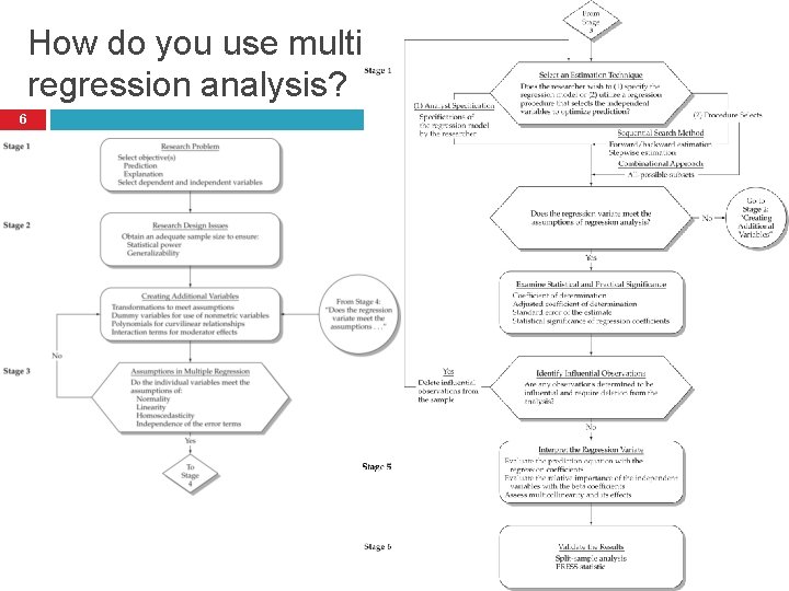
How do you use multiple regression analysis? 6

Simple vs. Multiple Regression 7 In general, the objective of regression analysis is to predict a single dependent variable from the knowledge of one or more independent variables. When the research problem involves a single independent variable, it is called simple regression. When the research problem involves two or more independent variables, it is called multiple regression.

8 STAGE 1: OBJECTIVES OF MULTIPLE REGRESSION

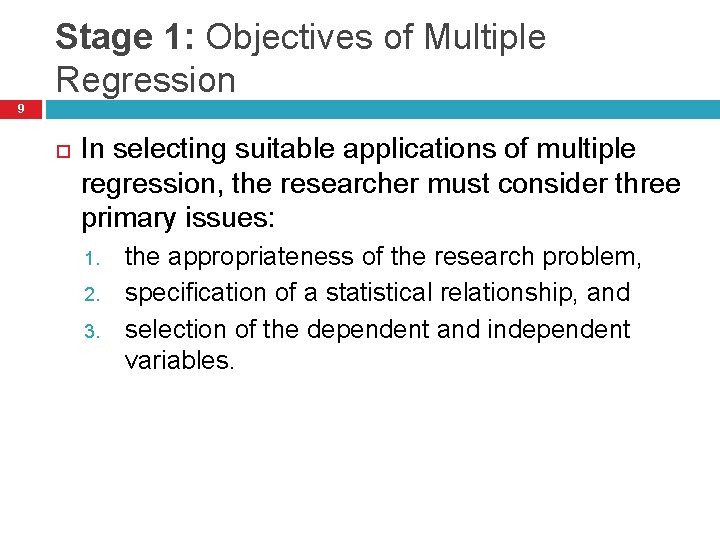
Stage 1: Objectives of Multiple Regression 9 In selecting suitable applications of multiple regression, the researcher must consider three primary issues: 1. 2. 3. the appropriateness of the research problem, specification of a statistical relationship, and selection of the dependent and independent variables.

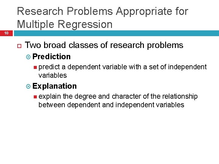
Research Problems Appropriate for Multiple Regression 10 Two broad classes of research problems Prediction predict a dependent variable with a set of independent variables Explanation explain the degree and character of the relationship between dependent and independent variables

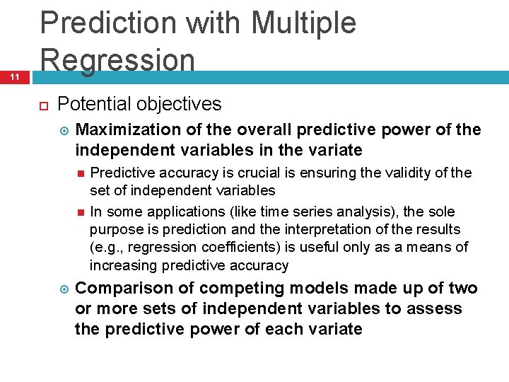
11 Prediction with Multiple Regression Potential objectives Maximization of the overall predictive power of the independent variables in the variate Predictive accuracy is crucial is ensuring the validity of the set of independent variables In some applications (like time series analysis), the sole purpose is prediction and the interpretation of the results (e. g. , regression coefficients) is useful only as a means of increasing predictive accuracy Comparison of competing models made up of two or more sets of independent variables to assess the predictive power of each variate

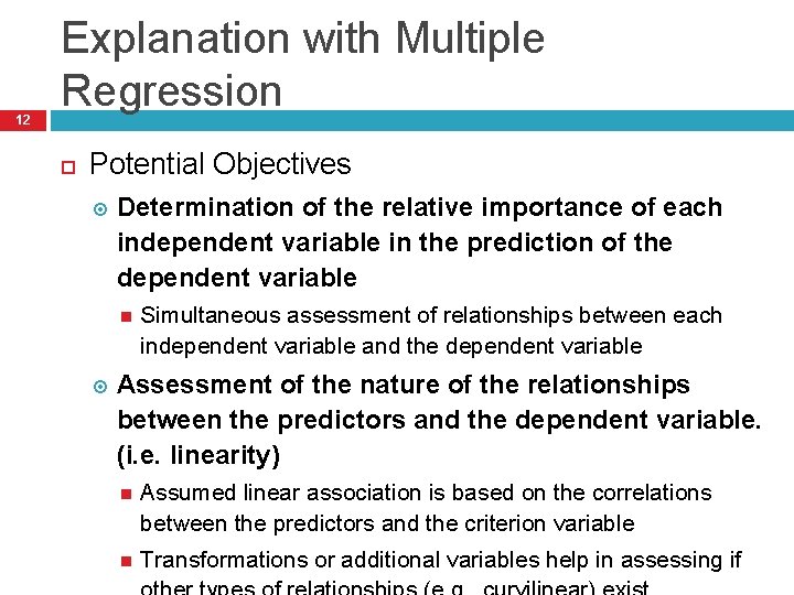
12 Explanation with Multiple Regression Potential Objectives Determination of the relative importance of each independent variable in the prediction of the dependent variable Simultaneous assessment of relationships between each independent variable and the dependent variable Assessment of the nature of the relationships between the predictors and the dependent variable. (i. e. linearity) Assumed linear association is based on the correlations between the predictors and the criterion variable Transformations or additional variables help in assessing if

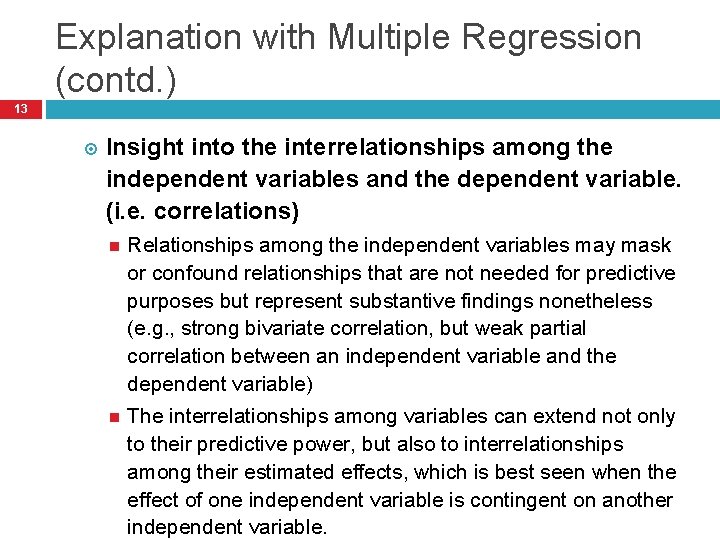
Explanation with Multiple Regression (contd. ) 13 Insight into the interrelationships among the independent variables and the dependent variable. (i. e. correlations) Relationships among the independent variables may mask or confound relationships that are not needed for predictive purposes but represent substantive findings nonetheless (e. g. , strong bivariate correlation, but weak partial correlation between an independent variable and the dependent variable) The interrelationships among variables can extend not only to their predictive power, but also to interrelationships among their estimated effects, which is best seen when the effect of one independent variable is contingent on another independent variable.

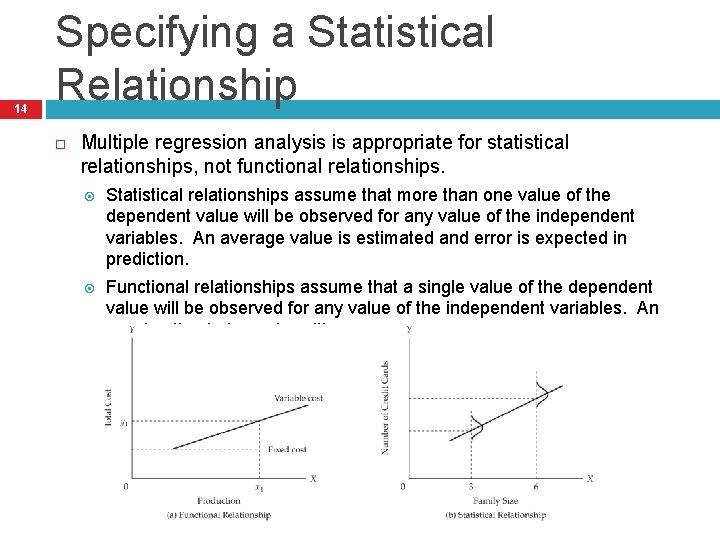
14 Specifying a Statistical Relationship Multiple regression analysis is appropriate for statistical relationships, not functional relationships. Statistical relationships assume that more than one value of the dependent value will be observed for any value of the independent variables. An average value is estimated and error is expected in prediction. Functional relationships assume that a single value of the dependent value will be observed for any value of the independent variables. An exact estimate is made, with no error.

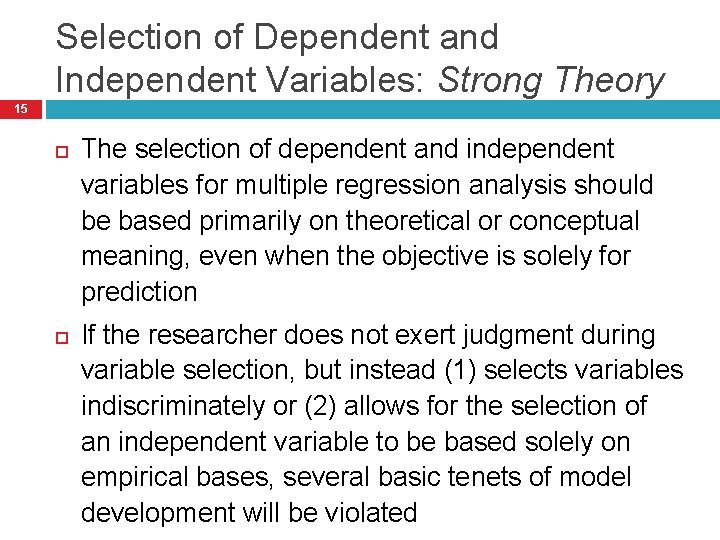
Selection of Dependent and Independent Variables: Strong Theory 15 The selection of dependent and independent variables for multiple regression analysis should be based primarily on theoretical or conceptual meaning, even when the objective is solely for prediction If the researcher does not exert judgment during variable selection, but instead (1) selects variables indiscriminately or (2) allows for the selection of an independent variable to be based solely on empirical bases, several basic tenets of model development will be violated

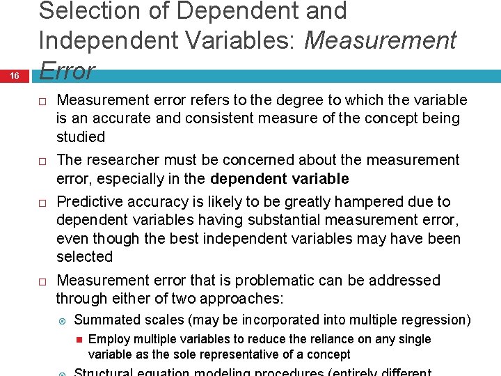
16 Selection of Dependent and Independent Variables: Measurement Error Measurement error refers to the degree to which the variable is an accurate and consistent measure of the concept being studied The researcher must be concerned about the measurement error, especially in the dependent variable Predictive accuracy is likely to be greatly hampered due to dependent variables having substantial measurement error, even though the best independent variables may have been selected Measurement error that is problematic can be addressed through either of two approaches: Summated scales (may be incorporated into multiple regression) Employ multiple variables to reduce the reliance on any single variable as the sole representative of a concept

17 Selection of Dependent and Independent Variables: Specification Error Most problematic issue in independent variable selection is specification error Inclusion of irrelevant variables Reduces model parsimony (i. e. , the fewest independent variables with the greatest contribution to the explained variance) The additional variables may mask or replace the effects of more useful variables The additional variables may make the statistical significance testing of the independent variables less precise and reduce the statistical and practical significance of the analysis Excluding relevant variables Can bias the results and negatively affect any interpretation of them (seriousness of bias depends on whether the omitted variables are correlated with the included variables or not)

18 Rules of Thumb 4 -1: Meeting Multiple Regression Objectives Only structural equation modeling (SEM) can directly accommodate measurement error, but using summated scales can mitigate it when using multiple regression. When in doubt, include potentially irrelevant variables (as they can only confuse interpretation) rather than possibly omitting a relevant variable (which can bias all regression estimates).

19 STAGE 2: RESEARCH DESIGN OF A MULTIPLE REGRESSION ANALYSIS

Stage 2: Research Design of a Multiple Regression Analysis 20 Three key features of multiple regression 1. 2. 3. Sample size: Multiple regression maintains the necessary levels of statistical power and practical/statistical significance across a broad range of sample sizes. Unique elements of the dependence relationship: Even though independent variables are assumed to be metric and have a linear relationship with the dependent variable, both assumptions can be relaxed by creating additional variables to represent these special aspects of the relationship. Nature of the independent variables: Multiple regression accommodates metric independent variables that are assumed to be fixed in nature as well as those with a random component.

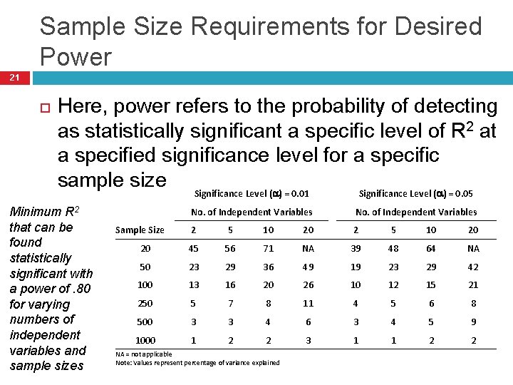
Sample Size Requirements for Desired Power 21 Here, power refers to the probability of detecting as statistically significant a specific level of R 2 at a specified significance level for a specific sample size Significance Level (a) = 0. 01 Significance Level (a) = 0. 05 Minimum R 2 that can be found statistically significant with a power of. 80 for varying numbers of independent variables and sample sizes No. of Independent Variables Sample Size 2 5 10 20 20 45 56 71 50 23 29 100 13 250 No. of Independent Variables 2 5 10 20 NA 39 48 64 NA 36 49 19 23 29 42 16 20 26 10 12 15 21 5 7 8 11 4 5 6 8 500 3 3 4 6 3 4 5 9 1000 1 2 2 3 1 1 2 2 NA = not applicable Note: Values represent percentage of variance explained

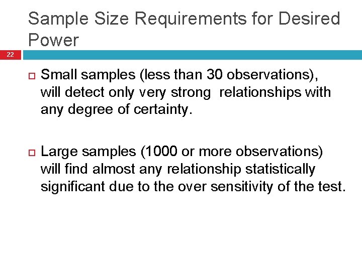
Sample Size Requirements for Desired Power 22 Small samples (less than 30 observations), will detect only very strong relationships with any degree of certainty. Large samples (1000 or more observations) will find almost any relationship statistically significant due to the over sensitivity of the test.

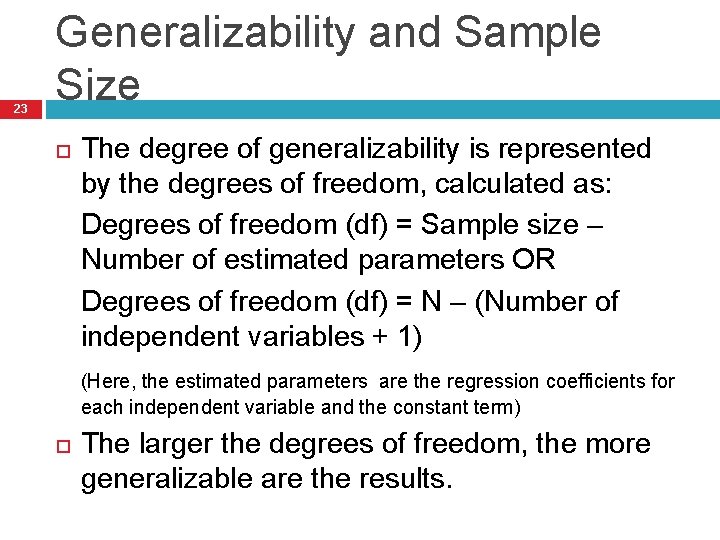
23 Generalizability and Sample Size The degree of generalizability is represented by the degrees of freedom, calculated as: Degrees of freedom (df) = Sample size – Number of estimated parameters OR Degrees of freedom (df) = N – (Number of independent variables + 1) (Here, the estimated parameters are the regression coefficients for each independent variable and the constant term) The larger the degrees of freedom, the more generalizable are the results.

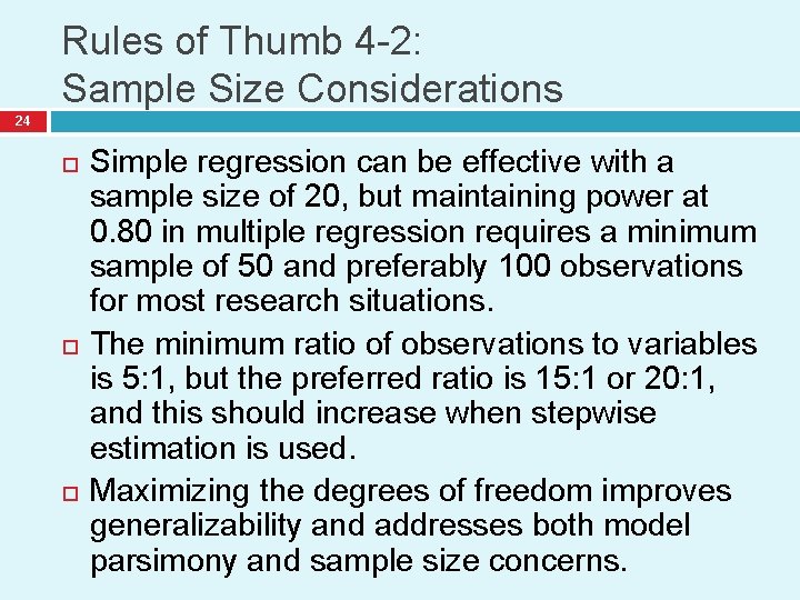
Rules of Thumb 4 -2: Sample Size Considerations 24 Simple regression can be effective with a sample size of 20, but maintaining power at 0. 80 in multiple regression requires a minimum sample of 50 and preferably 100 observations for most research situations. The minimum ratio of observations to variables is 5: 1, but the preferred ratio is 15: 1 or 20: 1, and this should increase when stepwise estimation is used. Maximizing the degrees of freedom improves generalizability and addresses both model parsimony and sample size concerns.

Creating Additional Variables 25 A researcher may desire to modify either the dependent or independent variables for one of two reasons: Improve or modify the relationship between the independent and dependent variables Enable the use of nonmetric variables in the regression variate Data transformations may be based on reasons that are either theoretical (transformation whose appropriateness is based on the nature of the data) or data derived (transformations that are suggested

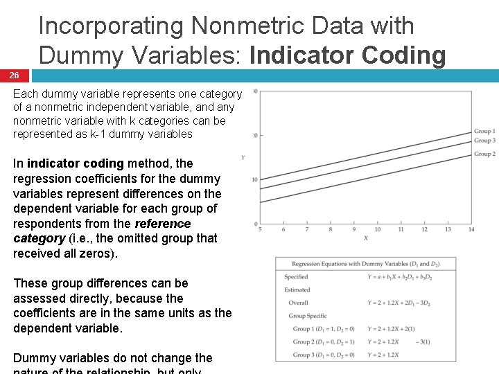
Incorporating Nonmetric Data with Dummy Variables: Indicator Coding 26 Each dummy variable represents one category of a nonmetric independent variable, and any nonmetric variable with k categories can be represented as k-1 dummy variables In indicator coding method, the regression coefficients for the dummy variables represent differences on the dependent variable for each group of respondents from the reference category (i. e. , the omitted group that received all zeros). These group differences can be assessed directly, because the coefficients are in the same units as the dependent variable. Dummy variables do not change the

Incorporating Nonmetric Data with Dummy Variables: Effects Coding 27 Effects coding is an alternative method of dummycoding It is the same as indicator coding, except that the comparison or omitted group is now given the value of -1 instead of 0 for the dummy variables Here, the regression coefficients for the dummy variables represent differences for any group from the mean of all groups (i. e. , the sample mean) rather than from the omitted group Both forms of dummy-variable coding will give the same results. The only differences will be in the interpretation of the dummy-variable coefficients.

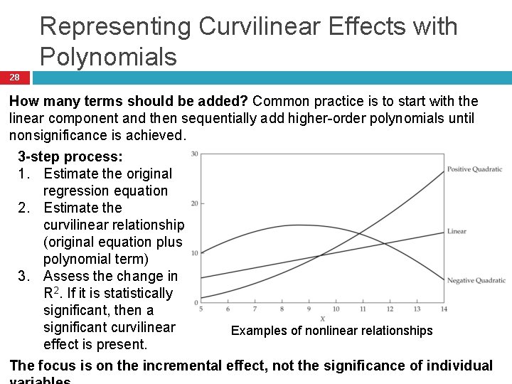
Representing Curvilinear Effects with Polynomials 28 How many terms should be added? Common practice is to start with the linear component and then sequentially add higher-order polynomials until nonsignificance is achieved. 3 -step process: 1. Estimate the original regression equation 2. Estimate the curvilinear relationship (original equation plus polynomial term) 3. Assess the change in R 2. If it is statistically significant, then a significant curvilinear Examples of nonlinear relationships effect is present. The focus is on the incremental effect, not the significance of individual

Representing Interaction or Moderator Effects 29 Moderator effect: Reflects the changing nature of one independent variable's relationship with the dependent variable as a function of another independent variable (called the moderator variable). Also known as the interaction effect. Example of moderator effect Quasi or bilinear moderator effect: The slope of the relationship of one independent variable (say, X 1) changes across values of the moderator variable (say, X 2). Moderator effects are represented as a compound variable (e. g. , X 1 X 2) in the regression equation. (e. g. , Y = b 0+ b 1 X 1 + b 2 X 2 + b 3 X 1 X 2 ) A 3 -step process of testing, similar to polynomials to represent nonlinear effects, is also followed here. Moderators change the interpretation of the regression coefficients. To determine the total effect of an independent variable, the separate and the moderated effects must be combined. (e. g. , b =

Rules of Thumb 4 -3: Variable Transformations 30 Nonmetric variables can only be included in a regression analysis by creating dummy variables. Dummy variables can only be interpreted in relation to their reference category with indicator coding format. Adding an additional polynomial term represents another inflection point in the curvilinear relationship. Quadratic and cubic polynomials are generally sufficient to represent most curvilinear relationships. Assessing the significance of a polynomial or interaction term is accomplished by evaluating incremental R 2, not the significance of individual coefficients, due to high multicollinearity.

31 STAGE 3: ASSUMPTIONS IN MULTIPLE REGRESSION ANALYSIS

Stage 3: Assumptions in Multiple Regression Analysis 32 The basic issue is: Are the errors in prediction a result of an actual absence of a relationship among the variables, or are they caused by some characteristics of the data not accommodated by the regression model? Assumptions are examined in five areas: Linearity of the phenomenon measured Constant variance of the error terms Independence of the error terms Normality of the error term distribution Multicollinearity

Assessing the Individual Variable versus the Variate 33 The derived variate in multiple regression acts collectively in predicting the dependent variable. Hence, it becomes necessary to assess the assumptions not only for individual variables, but also for the variate itself. The testing for assumptions for the variate are actually performed after the regression model has been estimated. The results from the individual variable assumption testing (performed in the initial phases of regression) can provide insights in areas such as: Have assumption violations for individual variable(s) caused their relationships to be misrepresented? What are the sources and remedies of any assumptions violations for the variate?

34 Methods of Diagnosis for the Variate Residual: The difference between the observed and predicted values for the dependent variable. It is a principle measure of prediction error for the variate. Studentized residual: Standardized form of the residuals, whose values correspond to t values. Plotting the residuals versus the independent or predicted variables is a basic method of identifying assumption violations for the overall relationship In multiple regression, unless the residual analysis intends to concentrate only on a single variable, the most common residual plot involves plotting the residuals (ri) against the predicted dependent values (Yi) (representing the total effect of the regression variate).

Graphical Analysis of Residuals 35

Linearity of the Phenomenon 36 The linearity of the relationship between dependent and independent variables represents the degree to which the change in the dependent variable is associated with the independent variable. Exhibited by a null plot. Possible corrective actions for assumption violation: Data transformation (e. g. , logarithm, square root, etc. ) of one or more independent variables Directly incorporating nonlinear relationships in the regression model (e. g. , creation of polynomial terms) Using specialized methods such as nonlinear regression Partial regression plots show the relationship of a single independent variable to the dependent variable, controlling for the effects of all other independent variables. Useful tool for determining which independent variable(s) to select for corrective action.

37 Constant Variance of the Error Term Homoscedasticity: The assumption is that the variance of the dependent variable values will be equal. Thus, for each level of the independent variable, the dependent variable should have a constant variance. Exhibited by a null plot. Heteroscedasticity: A condition referred to when the variance distributions are not equal. Possible corrective actions for assumption violation: Employ variance-stabilizing transformations Employ the procedure of weighted least squares, if the violation is attributed to a single independent variable Residual plots are primarily used for assessing this assumption. Statistical tests (e. g. , Levene test offered in SPSS) for homogeneity of variance are also available for nonmetric independent variables.

38 Independence of the Error Terms It is assumed that each predicted value is independent, implying that the predictions are not sequenced by any variable, i. e. , the researcher should expect the same chance of random error at each level of prediction. Plotting the residuals against any possible sequencing variable can reveal such occurrences If the residuals are independent, the pattern should appear random and similar to the null plot. Possible corrective actions for assumption violation: Data transformations (e. g. , first differences in a time series model) Inclusion of indicator variables (e. g. , seasonal indicator

39 Normality of the Error Distribution The data distribution for all variables is assumed to be the normal distribution. A normal distribution is necessary for the use of the F and t statistics, since sufficiently large violations of this assumption invalidate the use of these statistics. Diagnosis can be done using Normal probability plots of the residuals (preferred) Histogram of residuals Skewness tests

Multicollinearity 40 The presence of collinearity or multicollinearity suppresses the R 2 and confounds the analysis of the variate. This correlation among the predictor variables prohibits assessment of the contribution of each independent variable. Tolerance value or the variance inflation factor (VIF) can be used to detect multicollinearity. Once detected, the analyst may choose one of four options: omit the correlated variables, use the model for prediction only, assess the predictor-dependent variable relationship with simple correlations, or use a different method such as Bayesian regression.

Rules of Thumb 4 -4: Assessing Statistical Assumptions 41 Testing assumptions must be done not only for each dependent and independent variable, but for the variate as well. Graphical analyses (i. e. , partial regression plots, residual plots and normal probability plots) are the most widely used methods of assessing assumptions for the variate. Remedies for problems found in the variate must be accomplished by modifying (transforming) one or more independent variables.

42 STAGE 4: ESTIMATING THE REGRESSION MODEL AND ASSESSING THE OVERALL MODEL FIT

43 Stage 4: Estimating the Regression Model and Assessing the Overall Model Fit Major tasks in this stage: 1. 2. 3. 4. Selecting an estimation technique for specifying the regression model Testing the regression variate for meeting the regression assumptions Examining the statistical significance of the overall model Identifying influential observations

44 Selecting an Estimation Technique The basic issue is: Does the researcher wish to 1. specify the regression model? OR 2. Confirmatory Specification utilize a regression procedure that selects the independent variables to optimize prediction? Sequential Search Methods Combinatorial Approach

Confirmatory Specification 45 The analyst specifies the complete set of independent variables. Thus, the analyst has total control over variable selection. Although the confirmatory specification is conceptually simple, the researcher is completely responsible for the trade-offs between more independent variables and greater predictive accuracy versus model parsimony and concise explanation. The researcher must avoid being guided by empirical information and instead rely heavily on theoretical justification for a truly confirmatory

Sequential Search Methods 46 Sequential approaches estimate a regression equation with a set of variables defined by the researcher and by selectively adding or deleting among these variables until some overall criterion measure is achieved. This approach provides an objective method for selecting variables that maximizes the prediction while employing the smallest number of variables. Two types of sequential search approaches Stepwise elimination Forward addition and backward elimination

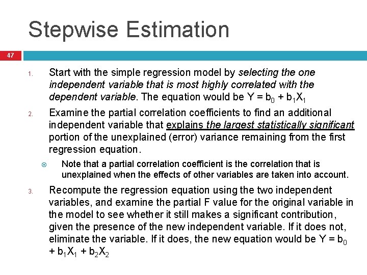
Stepwise Estimation 47 Start with the simple regression model by selecting the one independent variable that is most highly correlated with the dependent variable. The equation would be Y = b 0 + b 1 X 1 1. Examine the partial correlation coefficients to find an additional independent variable that explains the largest statistically significant portion of the unexplained (error) variance remaining from the first regression equation. 2. 3. Note that a partial correlation coefficient is the correlation that is unexplained when the effects of other variables are taken into account. Recompute the regression equation using the two independent variables, and examine the partial F value for the original variable in the model to see whether it still makes a significant contribution, given the presence of the new independent variable. If it does not, eliminate the variable. If it does, the new equation would be Y = b 0 + b 1 X 1 + b 2 X 2

Stepwise Estimation (continued) 48 4. 5. Continue this procedure by examining all independent variables not in the model to determine whether one would make a statistically significant addition to the current equation and thus should be included in a revised equation. If a new independent variable is included, examine all independent variables previously in the model to judge whether they should be kept or not. Continue adding independent variables until none of the remaining candidates for inclusion would contribute a statistically significant improvement in predictive accuracy. This point occurs when all of the

49 Forward and Backward Elimination The forward addition model is similar to the stepwise procedure in that it builds the regression equation starting with a single independent variable, whereas the backward elimination procedure starts with a regression equation including all the independent variables, and then deletes independent variables that do not contribute significantly. The primary distinction of the stepwise approach from these procedures is its ability to add or delete variables at each stage. Once a variable is added or deleted in the forward addition or backward

50 Caveats to Sequential Search Methods Multicollinearity among independent variables has substantial impact on the final model specification. E. g. , If two independent variables are highly correlated to each other as well as to the dependent variable, it is unlikely that both these variables will be included in the regression model through the stepwise approach. All sequential methods create a loss of control on the part of a researcher. In conducting the stepwise procedure, it is

Combinatorial Approach 51 The combinatorial approach estimates regression equations for all subset combinations of the independent variables. The most common procedure is known as all-possible-subsets regression. Some criticisms of this approach: For example, for even 10 independent variables, one would have to estimate 1024 regression equations. Atheoretical nature Lack of considerations such as multicollinearity, outliers, influential observations, and interpretability of results. Useful in providing insight into the number of regression models that are roughly equivalent in predictive power, yet possess quite different combinations of independent variables.

Rules of Thumb 4 -5: Estimation Techniques 52 No matter which estimation technique is chosen, theory must be a guiding factor in evaluating the final regression model because: Confirmatory Specification, the only method to allow direct testing of a pre-specified model, is also the most complex from the perspectives of specification error, model parsimony and achieving maximum predictive accuracy. Sequential search (e. g. , stepwise), while maximizing predictive accuracy, represents a completely “automated” approach to model estimation, leaving the researcher almost no control over the final model specification. Combinatorial estimation, while considering all possible models, still removes control from the researcher in terms of final model specification even though the researcher can view the set of roughly equivalent models in terms of predictive accuracy. No single method is “Best” and the prudent strategy is to use a combination of approaches to capitalize on the strengths of each to reflect theoretical basis of the research question.

Examining the Statistical Significance of the Overall Model 53 Coefficient of Determination (R 2) The coefficient of determination is a measure of the amount of variance in the dependent variable explained by the independent variable(s). A value of one 1 means perfect explanation (not encountered in reality due to ever present error). A value of. 91 means that 91% of the variance in the dependent variable is explained by the independent variables. The amount of variation explained by the regression model should be more than the variation explained by the average. Thus, R 2 should be greater than zero. R 2 is impacted by two facets of the data: The number of independent variables relative to the sample size See sample size discussion earlier. For this reason, analysts should use the adjusted coefficient of determination, which adjusts for inflation in R 2 from overfitting the data. The number of independent variables included in the analysis. As you increase the number of independent variables in the model, you increase the R 2 automatically because the sum of squared errors by regression begins to approach the sum of squared errors about the average.

Examining the Statistical Significance of the Overall Model 54 Standard error of the estimate is another measure of the accuracy of our predictions. It represents an estimate of the standard deviation of the actual dependent values around the regression line. Since this is a measure of variation about the regression line, the smaller the standard error, the better. F-test The F-test reported with the R 2 is a significance test of the R 2. This test indicates whether a significant amount (significantly different from zero) of variance was explained by the model.

Analyzing the Variate 55 The variate is the linear combination of independent variables used to predict the dependent variables. Analysis of the variate relates the respective contribution of each independent variable in the variate to the regression model. The researcher is informed as to which independent variable contributes the most to the variance explained and may make relative judgments between/among independent variables (using standardized coefficients

Testing the Regression Coefficients for Statistical Significance 56 The intercept (or constant term) should be tested for appropriateness for the predictive model. If the constant is not significantly different from zero, it should not be used for predictive purposes. The estimated coefficients should be tested to ensure that across all possible samples, the coefficient would be different from zero. The size of the sample will impact the stability of the regression coefficients. The larger the sample size, the more generalizable the estimated coefficients will be. An F-test may be used to test the appropriateness of the intercept and the regression coefficients.

59 Rules of Thumb 4 -6: Statistical Significance and Influential Observations Always ensure practical significance when using large sample sizes, as the model results and regression coefficients could be deemed irrelevant even when statistically significant due just to the statistical power arising from large sample sizes. Use the adjusted R 2 as your measure of overall model predictive accuracy. Statistical significance is required for a relationship to have validity, but statistical significance without theoretical support does not support validity.

60 STAGE 5: INTERPRETING THE REGRESSION VARIATE

Stage 5: Interpreting the Regression Variate 61 When interpreting the regression variate, the researcher evaluates the estimated regression coefficients for their explanation of the dependent variable and evaluates the potential impact of omitted variables.

Standardized Regression Coefficients (Beta Coefficients) 62 Regression coefficients must be standardized (i. e. computed on the same unit of measurement) in order to be able to directly compare the contribution of each independent variable to explanation of the dependent variable. Beta coefficients (the term for standardized regression coefficients) enable the researcher to examine the relative strength of each variable in the equation. For prediction, regression coefficients are not standardized and, therefore, are in their original units of measurement.

Multicollinearity 63 Multicollinearity is a data problem that can adversely impact regression interpretation by limiting the size of the R-squared and confounding the contribution of independent variables. For this reason, two measures, tolerance and VIF, are used to assess the degree of collinearity among independent variables.

Tolerance 64 Tolerance is a measure of collinearity between two independent variables or multicollinearity among three or more independent variables. It is the proportion of variance in one independent variable that is not explained by the remaining independent variables. Each independent variable will have a tolerance measure and each of measure should be close to 1. A tolerance of less than . 5 indicates a collinearity or multicollinearity problem.

Variance Inflation Factor (VIF) 65 Variance inflation factor (VIF) is the reciprocal of the tolerance value and measures the same problem of collinearity. VIF values of just over 1. 0 are desirable, with the floor VIF value being 1. 0. A VIF value of 1. 007 would be considered very good and indicative of no collinearity.

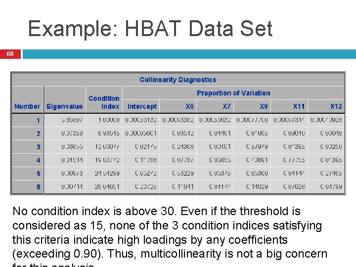
Assessing Multicollinearity with Condition Indices 66 The condition index represents the collinearity of combinations of variables in the data set (actually the relative size of the eigenvalues of the matrix … the condition indices are the square roots of the ratio of the largest eigenvalue to each individual eigenvalue). The regression coefficient variancedecomposition matrix shows the proportion of variance for each regression coefficient (and its associated variable) attributable to each

Assessing Multicollinearity with Condition Indices: A Two-Step Process 67 1. 2. Identify all condition indices above a threshold value. The threshold value usually is in the range of 15 to 30, with 30 the most commonly used value. For all condition indices exceeding the threshold, identify variables with variance proportions above 90%. A collinearity problem is indicated when a condition index identified in step 1 as above threshold value accounts for a substantial proportion of variance (0. 90 or above) for two or more

Example: HBAT Data Set 68 No condition index is above 30. Even if the threshold is considered as 15, none of the 3 condition indices satisfying this criteria indicate high loadings by any coefficients (exceeding 0. 90). Thus, multicollinearity is not a big concern

Rules of Thumb 4 -7: Interpreting the Regression Variate 69 Interpret the impact of each independent variable relative to the other variables in the model, as model respecification can have a profound effect on the remaining variables: Use beta weights when comparing relative importance among independent variables Regression coefficients describe changes in the dependent variable, but can be difficult in comparing across independent variables if the response formats vary Multicollinearity may be considered “good” when it reveals a suppressor effect, but generally it is viewed as harmful since increases in multicollinearity: Reduce the overall R 2 that can be achieved Confound estimation of the regression coefficients Negatively impact the statistical significance tests of coefficients Generally accepted levels of multicollinearity (tolerance values up to 0. 10, corresponding to a VIF of 10) should be decreased in smaller

70 STAGE 6: VALIDATION OF THE RESULTS

71 Stage 6: Validation of the Results 1. The researcher must ensure that the regression model represents the general population (generalizability) and is appropriate for the applications in which it will be employed (transferability). Collection of additional samples or split samples The regression model or equation may be retested on a new or split sample. No regression model should be assumed to be the final or absolute model of the population.

72 Stage 6: Validation of the Results 2. Calculation of the PRESS statistic Assesses the overall predictive accuracy of the regression by a series of iterations, whereby one observation is omitted in the estimation of the regression model and the omitted observation is predicted with the estimated model. The residuals for the observations are summed to provide an overall measure of predictive fit. 3. Comparison of regression models The adjusted R-square is compared across different estimated regression models to assess the model with the best prediction.

On Transferability of Regression Models 73 Before applying an estimated regression model to a new set of independent variable values, the researcher should consider the following: Predictions have multiple sampling variations, not only the sampling variations from the original sample, but also those of the newly drawn sample. Conditions and relationships should not have changed materially from their measurement at the time the original sample was taken. Do not use the model to estimate beyond the range of the independent variables in the sample. The regression equation is only valid for prediction purposes within the original range of magnitude for the prediction variables. Results cannot be extrapolated beyond the original range of variables measured since the form of the relationship may change.

Summary 74 1. 2. 3. 4. 5. 6. Determine when regression analysis is the appropriate statistical tool in analyzing a problem. Understand how regression helps us make predictions using the least squares concept. Use dummy variables with an understanding of their interpretation. Be aware of the assumptions underlying regression analysis and how to assess them. Select an estimation technique and explain the difference between stepwise and simultaneous regression. Interpret the results of regression.