Generalized Linear Models Generalized Linear Models GLM General

Generalized Linear Models

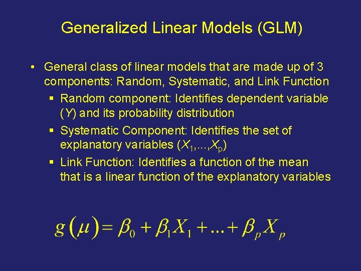
Generalized Linear Models (GLM) • General class of linear models that are made up of 3 components: Random, Systematic, and Link Function § Random component: Identifies dependent variable (Y) and its probability distribution § Systematic Component: Identifies the set of explanatory variables (X 1, . . . , Xp) § Link Function: Identifies a function of the mean that is a linear function of the explanatory variables

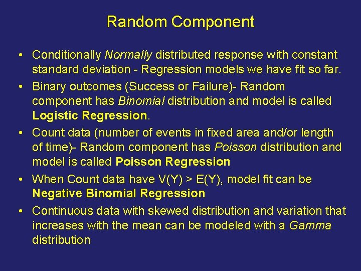
Random Component • Conditionally Normally distributed response with constant standard deviation - Regression models we have fit so far. • Binary outcomes (Success or Failure)- Random component has Binomial distribution and model is called Logistic Regression. • Count data (number of events in fixed area and/or length of time)- Random component has Poisson distribution and model is called Poisson Regression • When Count data have V(Y) > E(Y), model fit can be Negative Binomial Regression • Continuous data with skewed distribution and variation that increases with the mean can be modeled with a Gamma distribution

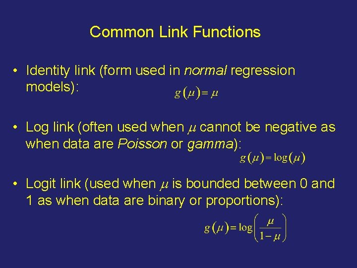
Common Link Functions • Identity link (form used in normal regression models): • Log link (often used when m cannot be negative as when data are Poisson or gamma): • Logit link (used when m is bounded between 0 and 1 as when data are binary or proportions):

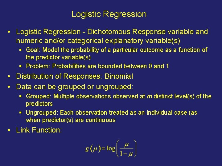
Logistic Regression • Logistic Regression - Dichotomous Response variable and numeric and/or categorical explanatory variable(s) § Goal: Model the probability of a particular outcome as a function of the predictor variable(s) § Problem: Probabilities are bounded between 0 and 1 • Distribution of Responses: Binomial • Data can be grouped or ungrouped: § Grouped: Multiple observations observed at m distinct level(s) of the predictors § Ungrouped: Each observation treated as an individual case (as when predictor(s) are continuous • Link Function:

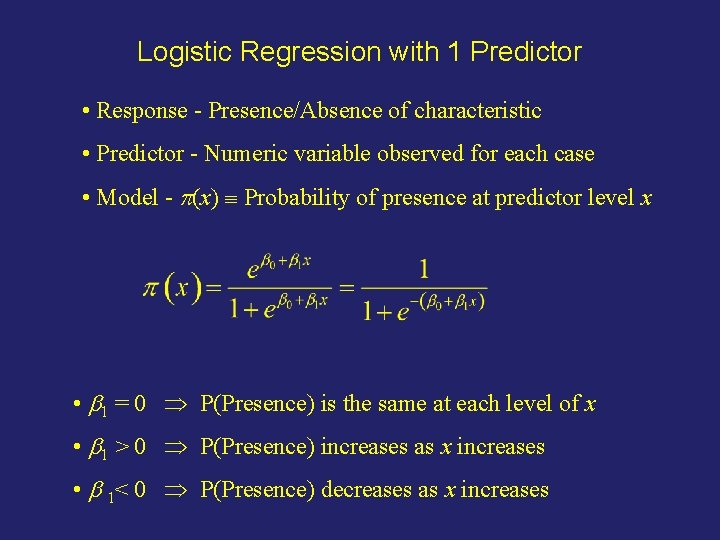
Logistic Regression with 1 Predictor • Response - Presence/Absence of characteristic • Predictor - Numeric variable observed for each case • Model - p(x) Probability of presence at predictor level x • b 1 = 0 P(Presence) is the same at each level of x • b 1 > 0 P(Presence) increases as x increases • b 1< 0 P(Presence) decreases as x increases

Model and Estimation

Model/Estimation – Null and Saturated Cases

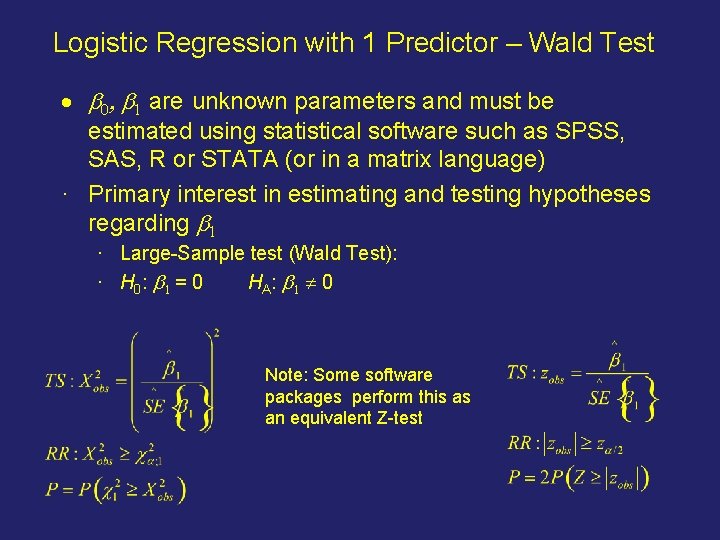
Logistic Regression with 1 Predictor – Wald Test · b 0, b 1 are unknown parameters and must be estimated using statistical software such as SPSS, SAS, R or STATA (or in a matrix language) · Primary interest in estimating and testing hypotheses regarding b 1 · Large-Sample test (Wald Test): · H 0 : b 1 = 0 HA: b 1 0 Note: Some software packages perform this as an equivalent Z-test

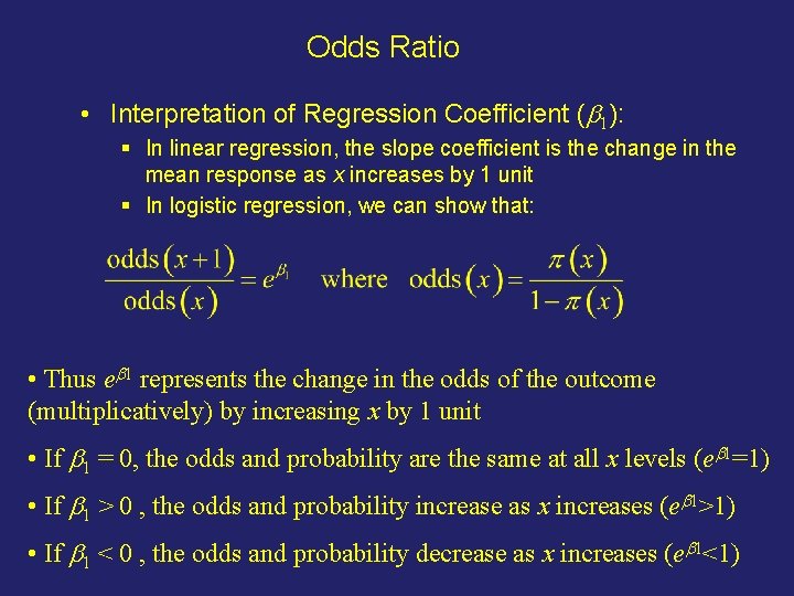
Odds Ratio • Interpretation of Regression Coefficient (b 1): § In linear regression, the slope coefficient is the change in the mean response as x increases by 1 unit § In logistic regression, we can show that: • Thus eb 1 represents the change in the odds of the outcome (multiplicatively) by increasing x by 1 unit • If b 1 = 0, the odds and probability are the same at all x levels (eb 1=1) • If b 1 > 0 , the odds and probability increase as x increases (eb 1>1) • If b 1 < 0 , the odds and probability decrease as x increases (eb 1<1)

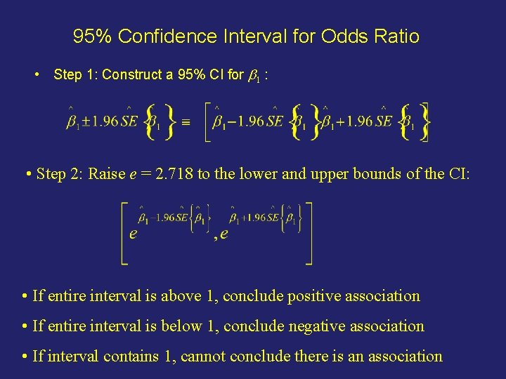
95% Confidence Interval for Odds Ratio • Step 1: Construct a 95% CI for b 1 : • Step 2: Raise e = 2. 718 to the lower and upper bounds of the CI: • If entire interval is above 1, conclude positive association • If entire interval is below 1, conclude negative association • If interval contains 1, cannot conclude there is an association

Likelihood Ratio Test / Deviance • The Wald Test is like the t-test in Linear Regression • The Likelihood Ratio Test is similar to the F-tests in Linear Regression

Residuals and Goodness-of-Fit Statistics

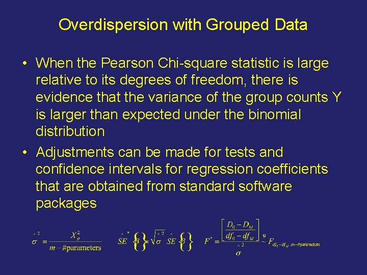
Overdispersion with Grouped Data • When the Pearson Chi-square statistic is large relative to its degrees of freedom, there is evidence that the variance of the group counts Y is larger than expected under the binomial distribution • Adjustments can be made for tests and confidence intervals for regression coefficients that are obtained from standard software packages

Pseudo-R 2 Statistics

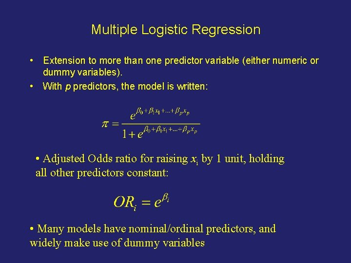
Multiple Logistic Regression • Extension to more than one predictor variable (either numeric or dummy variables). • With p predictors, the model is written: • Adjusted Odds ratio for raising xi by 1 unit, holding all other predictors constant: • Many models have nominal/ordinal predictors, and widely make use of dummy variables

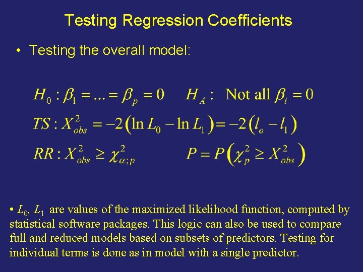
Testing Regression Coefficients • Testing the overall model: • L 0, L 1 are values of the maximized likelihood function, computed by statistical software packages. This logic can also be used to compare full and reduced models based on subsets of predictors. Testing for individual terms is done as in model with a single predictor.

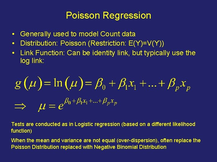
Poisson Regression • Generally used to model Count data • Distribution: Poisson (Restriction: E(Y)=V(Y)) • Link Function: Can be identity link, but typically use the log link: Tests are conducted as in Logistic regression (based on a different likelihood function) When the mean and variance are not equal (over-dispersion), often replace the Poisson Distribution replaced with Negative Binomial Distribution

Model and Estimation

Residuals and Goodness-of-Fit Statistics