Advanced applications of the GLM Crossfrequency coupling SPM

Advanced applications of the GLM: Cross-frequency coupling SPM course for MEG & EEG 2018 Bernadette van Wijk University of Amsterdam Department of Psychology University College London Wellcome Trust Centre for Neuroimaging

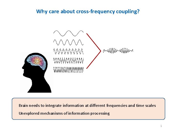
Why care about cross-frequency coupling? Brain needs to integrate information at different frequencies and time scales Unexplored mechanisms of information processing 1

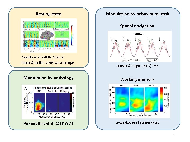
Resting state Modulation by behavioural task Spatial navigation Canolty et al. (2006) Science Florin & Baillet (2015) Neuroimage Jensen & Colgin (2007) Ti. CS Modulation by pathology Working memory de Hemptinne et al. (2013) PNAS Axmacher et al. (2009) PNAS 2

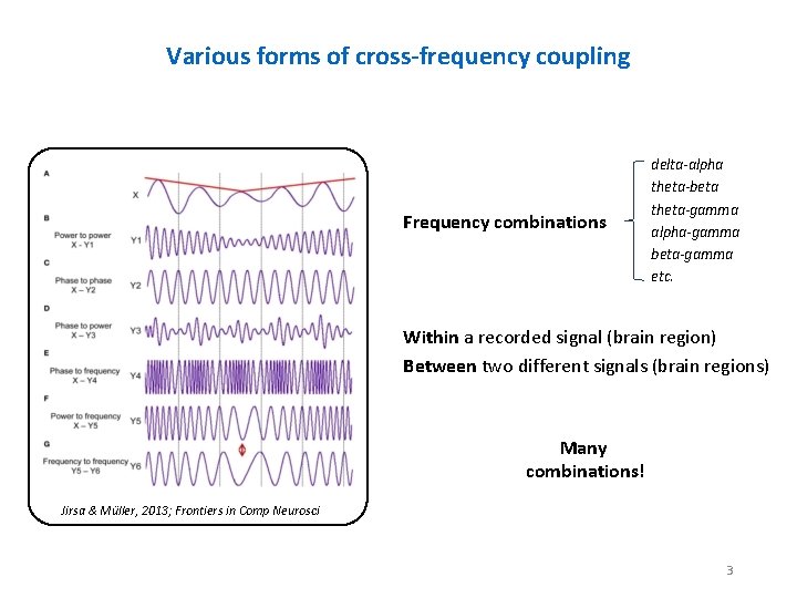
Various forms of cross-frequency coupling Frequency combinations delta-alpha theta-beta theta-gamma alpha-gamma beta-gamma etc. Within a recorded signal (brain region) Between two different signals (brain regions) Many combinations! Jirsa & Müller, 2013; Frontiers in Comp Neurosci 3

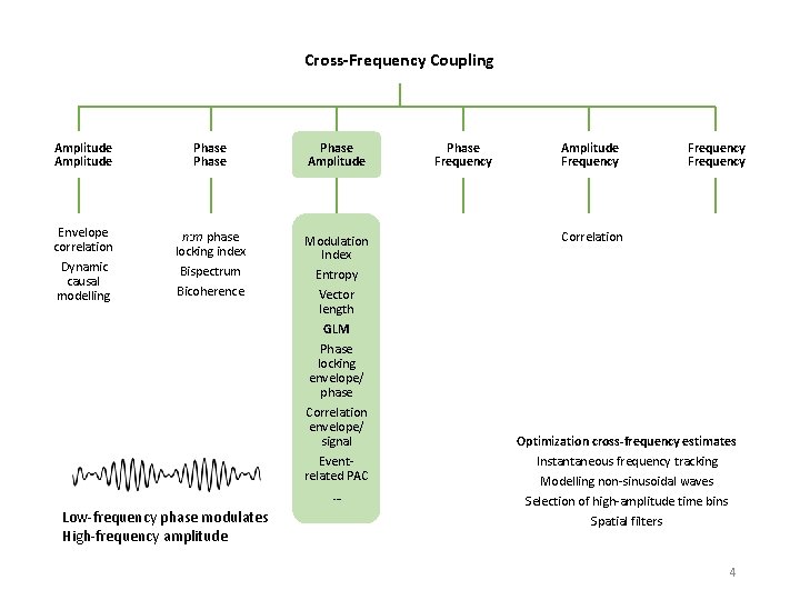
Cross-Frequency Coupling Amplitude Phase Amplitude Envelope correlation n: m phase locking index Modulation Index Entropy Vector length Dynamic causal modelling Bispectrum Bicoherence GLM Phase locking envelope/ phase Correlation envelope/ signal Eventrelated PAC … Low-frequency phase modulates High-frequency amplitude Phase Frequency Amplitude Frequency Correlation Optimization cross-frequency estimates Instantaneous frequency tracking Modelling non-sinusoidal waves Selection of high-amplitude time bins Spatial filters 4

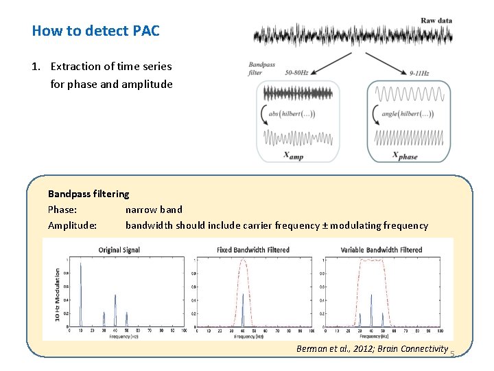
PAC: How to detect it How to detect PAC 1. Extraction of time series for phase and amplitude Bandpass filtering Phase: narrow band Amplitude: bandwidth should include carrier frequency ± modulating frequency Berman et al. , 2012; Brain Connectivity 5

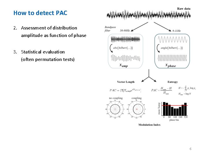
How to detect PAC 2. Assessment of distribution amplitude as function of phase 3. Statistical evaluation (often permutation tests) 6

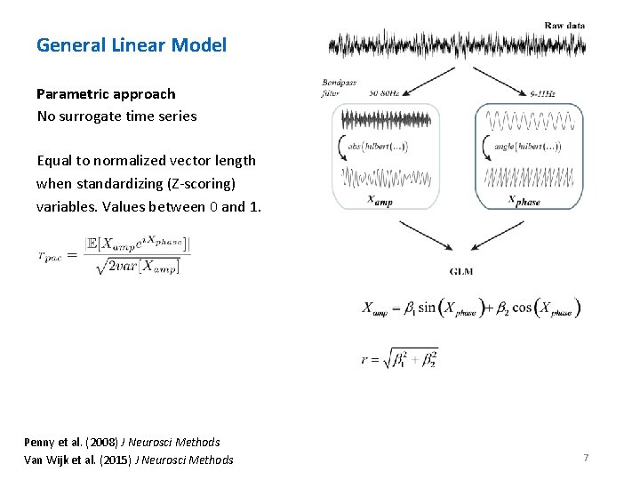
PAC: How to detect it General Linear Model Parametric approach No surrogate time series Equal to normalized vector length when standardizing (Z-scoring) variables. Values between 0 and 1. Penny et al. (2008) J Neurosci Methods Van Wijk et al. (2015) J Neurosci Methods 7

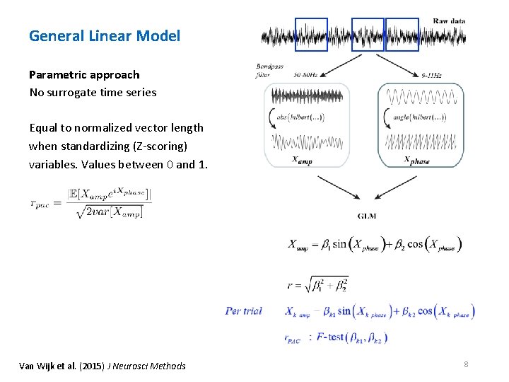
General Linear Model Parametric approach No surrogate time series Equal to normalized vector length when standardizing (Z-scoring) variables. Values between 0 and 1. Van Wijk et al. (2015) J Neurosci Methods 8

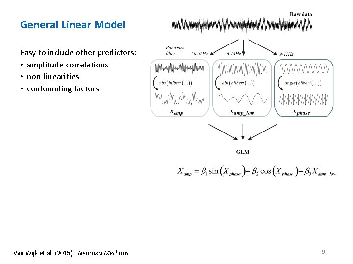
PAC: How to detect it General Linear Model Easy to include other predictors: • amplitude correlations • non-linearities • confounding factors Van Wijk et al. (2015) J Neurosci Methods 9

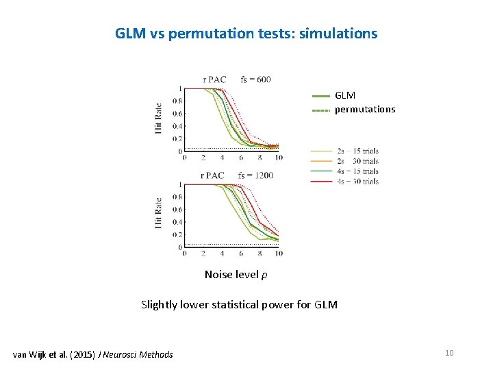
GLM vs permutation tests: simulations GLM permutations Noise level ρ Slightly lower statistical power for GLM van Wijk et al. (2015) J Neurosci Methods 10

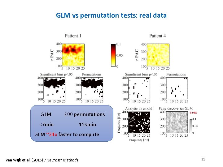
GLM vs permutation tests: real data GLM 200 permutations <7 min 159 min GLM ~24 x faster to compute van Wijk et al. (2015) J Neurosci Methods 11

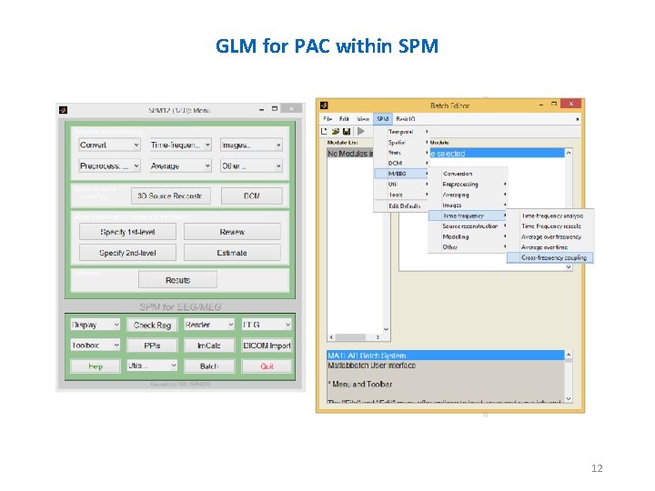
PAC: How to detect it GLM for PAC within SPM 12

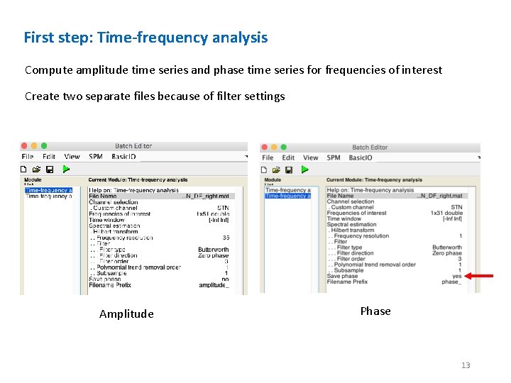
First step: Time-frequency analysis Compute amplitude time series and phase time series for frequencies of interest Create two separate files because of filter settings Amplitude Phase 13

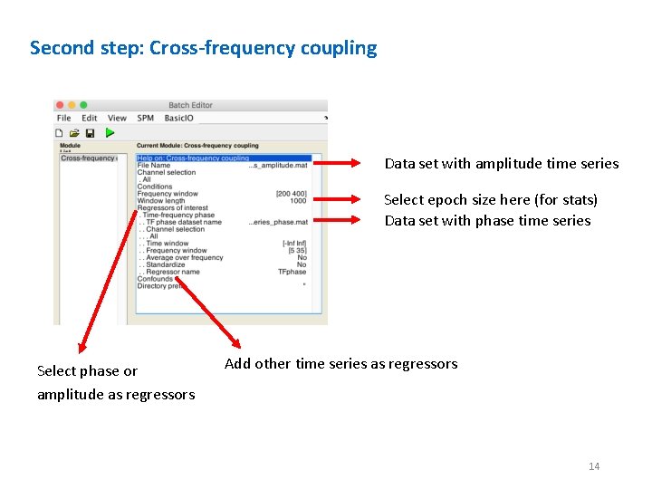
Second step: Cross-frequency coupling Data set with amplitude time series Select epoch size here (for stats) Data set with phase time series Select phase or amplitude as regressors Add other time series as regressors 14

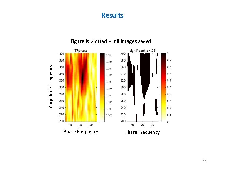
Results Amplitude Frequency Figure is plotted +. nii images saved Phase Frequency 15

Get in touch for an example batch and/or script: vanwijk. bernadette@gmail. com Or ask for help during the practical session on Wednesday 16