Generalized Linear Models GLM in R EPID 799

Generalized Linear Models (GLM) in R EPID 799 C Fall 2018 May want to pull down R code for today’s lecture from website. And a thanks to Nat and Sara for some previous slide content

Overview • Review of GLMs • Overview of R GLM functions • Accessing results • Comparison to SAS code

HW Notes • Tweaked the births_sm file – feel free to get again or use your own. May continue to tweak for class examples • Helper files (e. g. county tiers) you need for HW 3 are up on the site.

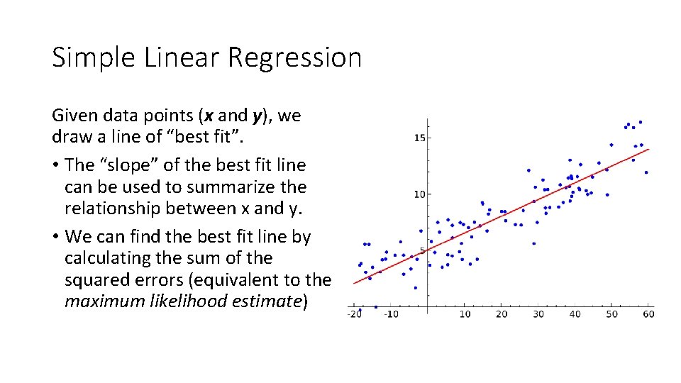
Simple Linear Regression Given data points (x and y), we draw a line of “best fit”. • The “slope” of the best fit line can be used to summarize the relationship between x and y. • We can find the best fit line by calculating the sum of the squared errors (equivalent to the maximum likelihood estimate)

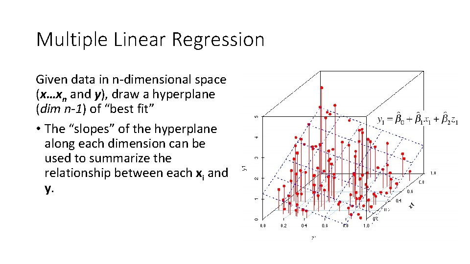
Multiple Linear Regression Given data in n-dimensional space (x…xn and y), draw a hyperplane (dim n-1) of “best fit” • The “slopes” of the hyperplane along each dimension can be used to summarize the relationship between each xi and y.

How the Computer Solves a Regression Except in trivial cases, a computer (through SAS, R, etc. ) uses the same painfully simple approach to determine the best line fit: 1. Choose a “guess” slope. 2. Calculate a fit statistic for the guess. (higher=worse, lower=better). 3. Repeat steps 1 and 2 until we find a “good” guess (a tolerance value defined by the user or set by default). [Optional Improvements] Keep track of your old guesses to see if you are getting “better” or “worse”. Have a system for selecting a good “jump” size between guesses. Start guessing somewhere that makes sense. Etc, etc.

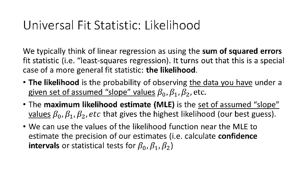
Universal Fit Statistic: Likelihood •

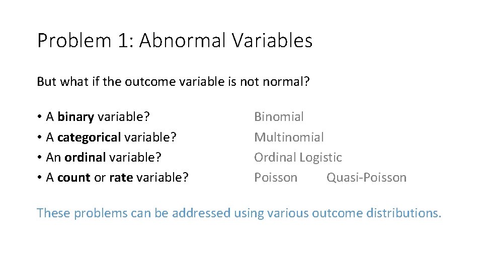
Problem 1: Abnormal Variables But what if the outcome variable is not normal? • A binary variable? • A categorical variable? • An ordinal variable? • A count or rate variable? Binomial Multinomial Ordinal Logistic Poisson Quasi-Poisson These problems can be addressed using various outcome distributions.

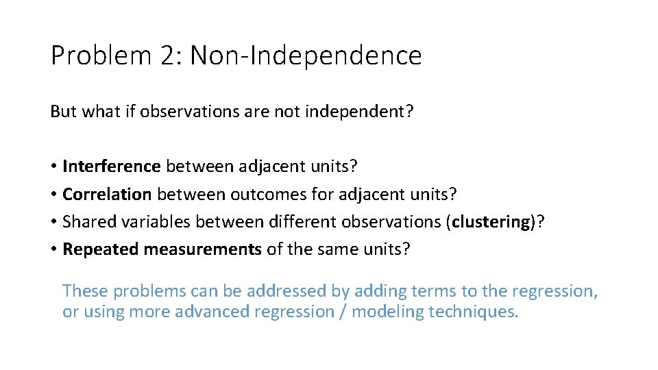
Problem 2: Non-Independence But what if observations are not independent? • Interference between adjacent units? • Correlation between outcomes for adjacent units? • Shared variables between different observations (clustering)? • Repeated measurements of the same units? These problems can be addressed by adding terms to the regression, or using more advanced regression / modeling techniques.

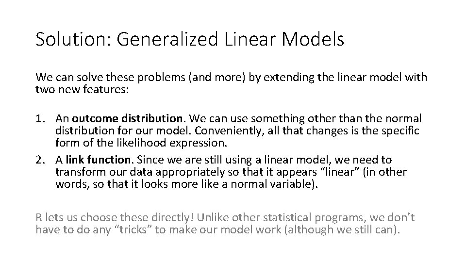
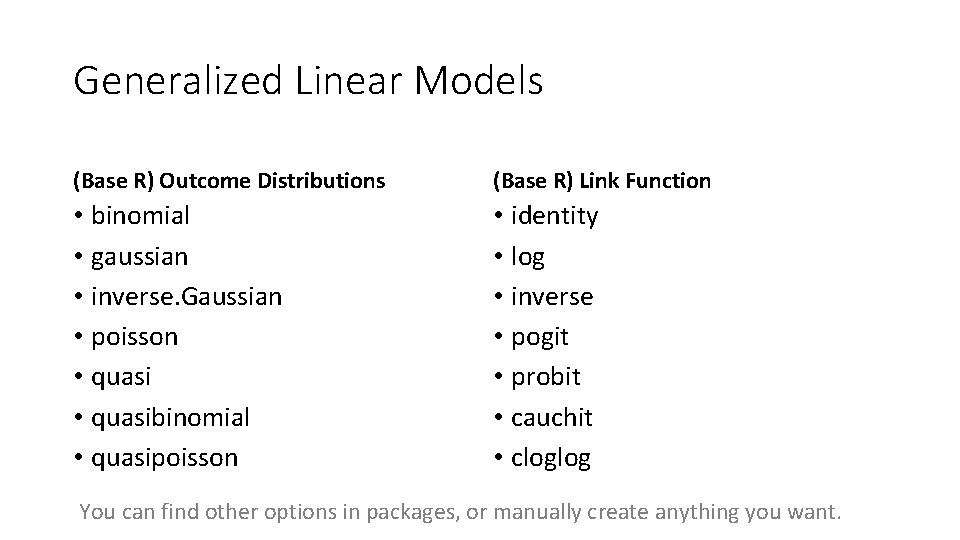
Solution: Generalized Linear Models We can solve these problems (and more) by extending the linear model with two new features: 1. An outcome distribution. We can use something other than the normal distribution for our model. Conveniently, all that changes is the specific form of the likelihood expression. 2. A link function. Since we are still using a linear model, we need to transform our data appropriately so that it appears “linear” (in other words, so that it looks more like a normal variable). R lets us choose these directly! Unlike other statistical programs, we don’t have to do any “tricks” to make our model work (although we still can).

Generalized Linear Models (Base R) Outcome Distributions (Base R) Link Function • binomial • gaussian • inverse. Gaussian • poisson • quasibinomial • quasipoisson • identity • log • inverse • pogit • probit • cauchit • cloglog You can find other options in packages, or manually create anything you want.

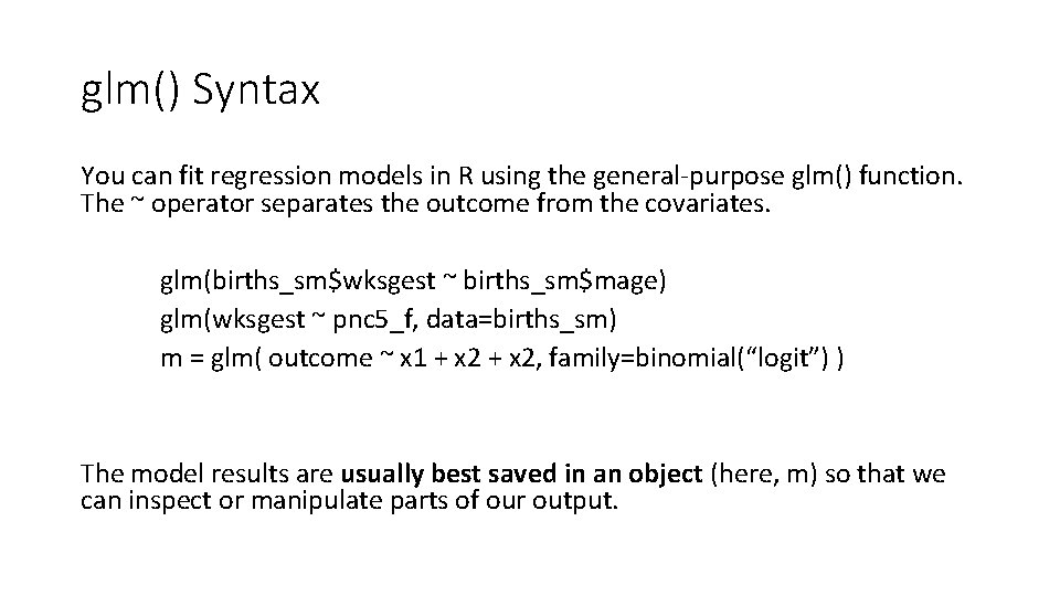
glm() Syntax You can fit regression models in R using the general-purpose glm() function. The ~ operator separates the outcome from the covariates. glm(births_sm$wksgest ~ births_sm$mage) glm(wksgest ~ pnc 5_f, data=births_sm) m = glm( outcome ~ x 1 + x 2, family=binomial(“logit”) ) The model results are usually best saved in an object (here, m) so that we can inspect or manipulate parts of our output.

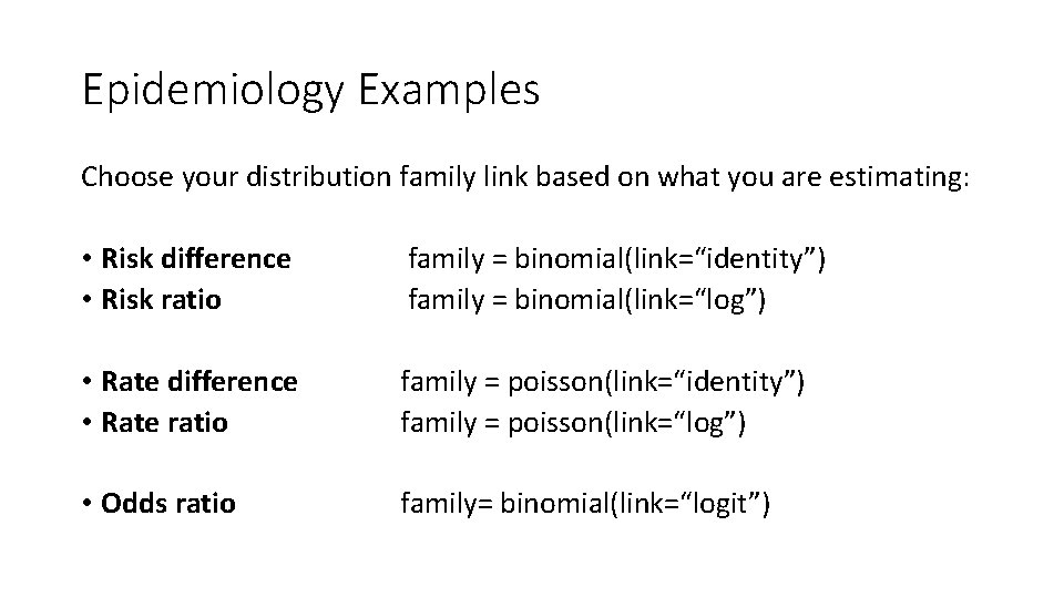
Epidemiology Examples Choose your distribution family link based on what you are estimating: • Risk difference • Risk ratio family = binomial(link=“identity”) family = binomial(link=“log”) • Rate difference • Rate ratio family = poisson(link=“identity”) family = poisson(link=“log”) • Odds ratio family= binomial(link=“logit”)

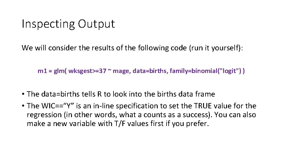
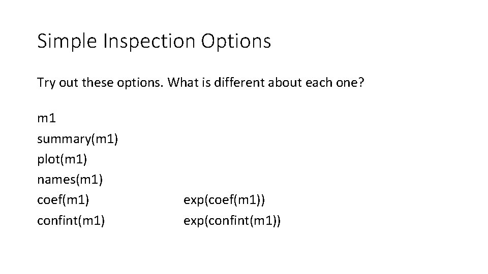
Inspecting Output We will consider the results of the following code (run it yourself): m 1 = glm( wksgest>=37 ~ mage, data=births, family=binomial("logit") ) • The data=births tells R to look into the births data frame • The WIC==“Y” is an in-line specification to set the TRUE value for the regression (in other words, what a counts as a success). You can also make a new variable with T/F values first if you prefer.

Simple Inspection Options Try out these options. What is different about each one? m 1 summary(m 1) plot(m 1) names(m 1) coef(m 1) confint(m 1) exp(coef(m 1)) exp(confint(m 1))

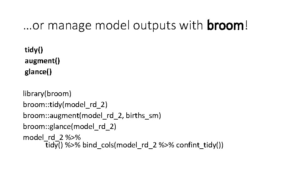
…or manage model outputs with broom! tidy() augment() glance() library(broom) broom: : tidy(model_rd_2) broom: : augment(model_rd_2, births_sm) broom: : glance(model_rd_2) model_rd_2 %>% tidy() %>% bind_cols(model_rd_2 %>% confint_tidy())

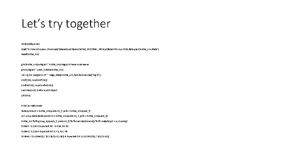
Let’s try together library(tidyverse) load("D: /User/Dropbox (Personal)/Education/Classes/18 Fall_EPID 799 C_Rfor. Epi/data/R for epi 2018 data pack/births_sm. rdata") head(births_sm) glm(births_sm$wksgest ~ births_sm$mage) # linear continuous glm(wksgest ~ pnc 5_f, data=births_sm) m 1 = glm( wksgest>=37 ~ mage, data=births_sm, family=binomial("logit") ) coef(m 1); exp(coef(m 1)) confint(m 1); exp(confint(m 1)) summary(m 1) # also a plot object plot(m 1) # Get a crude sense table(preterm = births_sm$preterm_f, pct 5 = births_sm$pnc 5_f) pt = prop. table(preterm = births_sm$preterm_f, pct 5 = births_sm$pnc 5_f)) births_sm %>% group_by(pnc 5_f, preterm_f) %>% summarize(n=n()) %>% mutate(pct = n / sum(n)) 0. 0943 - 0. 128 # Expected RD: -0. 034, R 1 -R 0 0. 0943 / 0. 128 # Expected RR: 0. 73, R 1 / R 0 (0. 0943 / (1 -0. 0943)) / (0. 128/(1 -0. 128)) # Expected OR: 0. 10 (R 0/(R)) / (R 1/(1 -R 1))

Let’s try together May want to pull down R code for today’s lecture from website.