Effect Measure Modification EPID 799 C Fall 2018

Effect Measure Modification EPID 799 C Fall 2018

Today A continuation of modeling: How do we get group-specific effect estimates and confidence intervals from models when we have EMM? Also: a recursion primer

Review 1. We’ve looked at a Directed Acyclic Graph to identify model covariates to control to assess the causal relationship of early prenatal care on preterm birth. We know EMM won’t show up on the DAG. 2. We’ve constructed Generalized Linear Models for risk difference (also looked at RRs and ORs) without EMM. 3. We’ve looked at crude EMM using dplyr: : and table(). Moderate modification? 4. Now we want modeled, stratum-specific effect estimates and CIs controlling for our other covariates (smoking, maternal age). We want a full EMM model.

Model Specification 1: Crude •

Model Specification 2 •

Model Specification 3 •

Model Specification 3 •

Full Model Specification w/ EMM •

Coding schemes • R’s default for expanding unordered factors in a model is indicator coding: R breaks up factors in models to all be referent to the baseline, meaning you need n-1 levels to describe n levels of a factor.

Let’s Look: Contrast Matrix

Full Model Specification w/ EMM •

Full Model Specification w/ EMM •

Contrasts •

We can get these point-estimates by hand a few ways… # Point estimates by hand, a few ways mfull_emm_rd$coefficients[2] #Wn. H RD_Wn. H = mfull_emm_rd$coefficients["pnc 5_f. PNC starts in first 5 mo"] #Wn. H RD_Wn. H + mfull_emm_rd$coefficients["pnc 5_f. PNC starts in first 5 mo: raceeth_f. AA"] #AA sum(mfull_emm_rd$coefficients[c(2, 10)]) # AA sum(mfull_emm_rd$coefficients[c(2, 11)]) # WH sum(coef(mfull_emm_rd)[c(2, 12)]) # AI/AN sum(coef(mfull_emm_rd)[c(2, 13)]) # Other

…But what about the CIs?

Contrast Package Lets you define arbitrary contrasts across your model that you’re interested in by setting two coefficient specifications as lists. contrast(<MODEL OBJECT>, a=list(<COEFA>), b=list(<COEFB>) Handles more than GLMs – also multi-level/LME, gee, etc. If you need exponentiated estimates, pass in fun=exp. See help page

Contrast Package: Example 1 For our full model… contrast(mfull_emm_rd, a=list(pnc 5_f = "PNC starts in first 5 mo", raceeth_f = "AA", smoker_f =”Non smoker”, mage=0, mage_sq=0), b=list(pnc 5_f = "No PNC before 5 mo", raceeth_f = "AA", smoker_f=“Non smoker”, mage=0, mage_sq=0)) Gets us the RD effect estimate and 95% CI for AA moms getting prenatal care vs. those who aren’t. Note that unchanging model levels are required to have something, but “drop out” of the estimation. This is similar to how predict() works.

Contrast Package: Example 2 For all levels of EMM: raceeth_diff = contrast(mfull_emm_rd, a=list(pnc 5_f = "PNC starts in first 5 mo", raceeth_f = levels(births$raceeth_f), smoker_f = “non Smoker", mage=0, mage_sq=0), b=list(pnc 5_f = "No PNC before 5 mo", raceeth_f = levels(births$raceeth_f), smoker_f=“non Smoker", mage=0, mage_sq=0)) print(raceeth_diff, X=T) Gets us the RD effect estimate and 95% CI for all levels of race-ethnicity including referent. Can use data. frame() to piece together a results table for graphing.

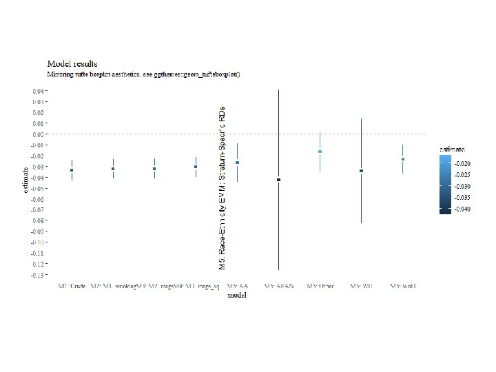
Let’s Try: Contrasts #. . . # EMM / final model #. . . glm(data=births, preterm_f ~ pnc 5_f + smoker_f, family=binomial(link="identity")) #Discussion of model spec head(births) table(births$race_f, births$methnic) # note my "ethnicity" coding may not be ideal. mfull_emm_rd = glm(data=births, preterm_f ~ pnc 5_f * raceeth_f + smoker_f + mage_sq, family=binomial(link="identity")) summary(mfull_emm_rd) broom: : tidy(mfull_emm_rd) # Point estimates by hand, a few ways mfull_emm_rd$coefficients[2] #Wn. H RD_Wn. H = mfull_emm_rd$coefficients["pnc 5_f. PNC starts in first 5 mo"] #Wn. H RD_Wn. H + mfull_emm_rd$coefficients["pnc 5_f. PNC starts in first 5 mo: raceeth_f. AA"] #AA sum(mfull_emm_rd$coefficients[c(2, 10)]) # AA sum(mfull_emm_rd$coefficients[c(2, 11)]) # WH sum(coef(mfull_emm_rd)[c(2, 12)]) # AI/AN sum(coef(mfull_emm_rd)[c(2, 13)]) # Other C(births$raceeth_f) # get or set contrasts(births$raceeth_f) # Let's look: contrast matrix # See contr. treatment or contr. sum # Contrasts using contrast package library(contrast) contrast(mfull_emm_rd, a=list(pnc 5_f = "PNC starts in first 5 mo", raceeth_f = "AA", smoker_f = "Smoker", mage=20, mage_sq=400), b=list(pnc 5_f = "No PNC before 5 mo", raceeth_f = "AA", smoker_f="Smoker", mage=20, mage_sq=400)) raceeth_diff = contrast(mfull_emm_rd, a=list(pnc 5_f = "PNC starts in first 5 mo", raceeth_f = levels(births$raceeth_f), smoker_f = "Smoker", mage=20, mage_sq=400), b=list(pnc 5_f = "No PNC before 5 mo", raceeth_f = levels(births$raceeth_f), smoker_f="Smoker", mage=20, mage_sq=400)) print(raceeth_diff, X=T) EMM_df = data. frame(model=paste 0("M 5: ", raceeth_diff$raceeth_f), estimate=raceeth_diff$Contrast, std. error = raceeth_diff$SE, X 2. 5. . =raceeth_diff$Lower, X 97. 5. . =raceeth_diff$Upper) ggplot(bind_rows(model_results, EMM_df), aes(model, estimate, color=std. error, fill=std. error))+ geom_linerange(aes(ymin=X 2. 5. . , ymax=X 97. 5. . ), size=1)+ geom_point(shape=15, size=4, color="white")+ geom_point(shape=15)+ scale_y_continuous(limits=c(NA, NA), breaks=seq(-0. 15, 0. 01))+ geom_hline(yintercept = 0, lty=2, color="grey")+ geom_vline(xintercept = 4. 5, lty=2, color="blue")+ annotate(geom = "text", x = 4. 6, y=-0. 05, angle=90, label="M 5: Race-Ethnicity EMM: Stratum-Specific RDs")+ labs(title="Model results", subtitle="Mirroring tufte boxplot aesthetics, see ggthemes: : geom_tufteboxplot()")+ ggthemes: : theme_tufte()

Other ways Specifying the contrast type using functions like: C() : Sets the "contrasts" attribute for the factor. contrasts(): Set and view the contrasts associated with a factor. model. matrix() : creates a design (or model) matrix, e. g. , by expanding factors to a set of dummy variables (depending on the contrasts) and expanding interactions similarly. Create a custom contrast matrix so that individual coefficients are more meaningful under EMM. Possible but beyond scope of this class. Good luck.

References A (sort of) complete guide to contrasts in R http: //rstudio-pubs-static. s 3. amazonaws. com/65059_586 f 394 d 8 eb 84 f 84 b 1 baaf 56 ffb 6 b 47 f. html contrast package https: //cran. r-project. org/web/packages/contrast/vignettes/contrast. pdf

Recursion The B in Benoit B Mandelbrot stands for Benoit B Mandelbrot.

Recursion In order to understand recursion you must first understand recursion. why are these bad examples of useful recursion?

• Use recursion if on each iteration your task splits into two or more similar tasks https: //stackoverflow. com/questions/126756/examples-of-recursivefunctions • …SMALLER tasks • …has reasonable base cases / terminating conditions • …is typically of unknown length / complexity

Typical teaching examples from computer science • Sorts galore • Tree traversal • Scheme / lists • …but what about public health?

A question on time clusters Hospital arrivals within 15 minutes apart become part of a cluster… including anyone time-adjacent to their own “time neighbors. ” (May not actually be Nidia’s question, but caught my attention as a good example…) Toy example: How many time clusters in h = c(1, 2, 4, 5, 6, 7, 10, 11, 13, 27)

Factorial, a classic! my_factorial = function(n, verbose=F){ if(n == 0) { if(verbose){print(" = ")} return(1) } else{ if(verbose){print(paste 0(n, " x"))} return(n * my_factorial(n-1, verbose)) } } my_factorial(5) my_factorial(5, verbose = T)

Now, some cluster finding library(tidyverse) h = c(1, 2, 4, 5, 6, 7, 10, 11, 13, 27) cluster_maker = function(a, b, d = 1 , found_list = NULL, verbose = F){ # a = 4; b=h; d=1; found_list=NULL if (verbose) {print(cat("Called with a=", a, "b=", b, "d=", d, "found= ", found_list))} # if starting, find myself! Then remove myself from rest of list if(is. null(found_list)){ found_list = a } rest_of_list = b[!(b %in% found_list)] # Reduce! # Find new matches, if I haven't seen them before, and add to found list new_matches = b[abs(a-b)<=d] new_matches = new_matches[!(new_matches %in% found_list)] found_list = c(new_matches, found_list) # for loop version child_answers = NULL # collect my children results 1 by 1 for(new_find in new_matches){ # more traditional would be first of list, rest of list child_answers = c(child_answers, cluster_maker(new_find, rest_of_list, d, found_list)) } # Could also unlist(map. . . ) instead of a loop found_list = found_list %>% union(child_answers) %>% `[`(order(. )) # ^ FANCY! Just merge and sort. return(found_list) # returns my results plus children results } h cluster_maker(1, cluster_maker(2, cluster_maker(4, cluster_maker(5, cluster_maker(7, h, h, h, 1) 1) 1, verbose = T) 1) 2)

More purrr practice! results_df = tibble(cluster_list = map(h, ~ cluster_maker(. x, h, 1)), cluster_lengths = map_int(cluster_list, length), cluster_id = map_chr(cluster_list, ~ paste(. x, collapse = " "))) length(unique(results_df$cluster_id))

Critical Thinking Might there be creative O(1)* ways to do this? h = c(1, 2, 4, 5, 6, 7, 10, 11, 13, 27) I think so!!