Measure Phase Welcome to Measure Welcome to Measure

Measure Phase Welcome to Measure

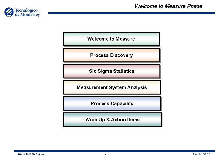
Welcome to Measure Phase Welcome to Measure Process Discovery Six Sigma Statistics Measurement System Analysis Process Capability Wrap Up & Action Items Green Belt Six Sigma 2 Fuente: OSSS

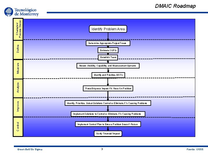
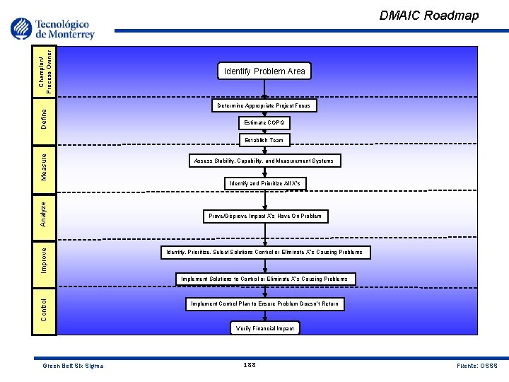
Champion/ Process Owner DMAIC Roadmap Identify Problem Area Define Determine Appropriate Project Focus Estimate COPQ Improve Analyze Measure Establish Team Assess Stability, Capability, and Measurement Systems Identify and Prioritize All X’s Prove/Disprove Impact X’s Have On Problem Identify, Prioritize, Select Solutions Control or Eliminate X ’s Causing Problems Control Implement Solutions to Control or Eliminate X ’s Causing Problems Implement Control Plan to Ensure Problem Doesn ’t Return Verify Financial Impact Green Belt Six Sigma 3 Fuente: OSSS

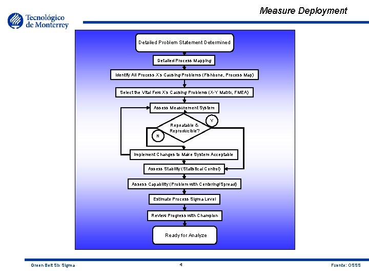
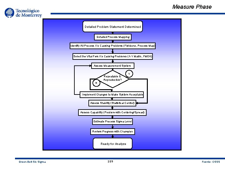
Measure Deployment Detailed Problem Statement Determined Detailed Process Mapping Identify All Process X’s Causing Problems (Fishbone, Process Map) Select the Vital Few X’s Causing Problems (X-Y Matrix, FMEA) Assess Measurement System N Repeatable & Reproducible? Y Implement Changes to Make System Acceptable Assess Stability (Statistical Control) Assess Capability (Problem with Centering/Spread) Estimate Process Sigma Level Review Progress with Champion Ready for Analyze Green Belt Six Sigma 4 Fuente: OSSS

Measure Phase Process Discovery

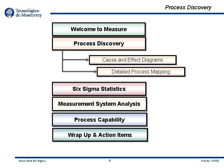
Process Discovery Welcome to Measure Process Discovery Cause and Effect Diagrams Detailed Process Mapping Six Sigma Statistics Measurement System Analysis Process Capability Wrap Up & Action Items Green Belt Six Sigma 6 Fuente: OSSS

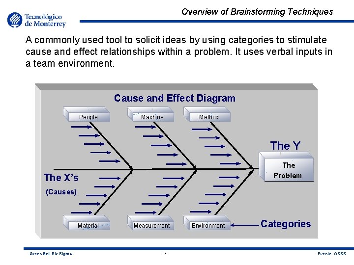
Overview of Brainstorming Techniques A commonly used tool to solicit ideas by using categories to stimulate cause and effect relationships within a problem. It uses verbal inputs in a team environment. Cause and Effect Diagram People Machine Method The Y The or Problem Condition The X’s (Causes) l Material Green Belt Six Sigma Measurement 7 Environment Categories Fuente: OSSS

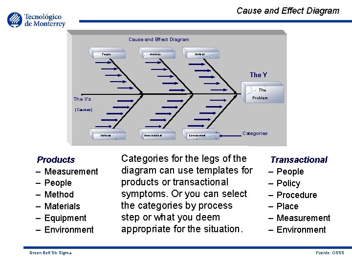
Cause and Effect Diagram People Machine Method The Y Theor Problem Condition The X’s (Causes) Material l Products – Measurement – People – Method – Materials – Equipment – Environment Green Belt Six Sigma Measurement Environment Categories for the legs of the diagram can use templates for products or transactional symptoms. Or you can select the categories by process step or what you deem appropriate for the situation. Transactional – People – Policy – Procedure – Place – Measurement – Environment Fuente: OSSS

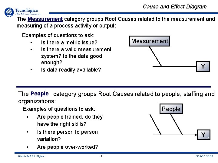
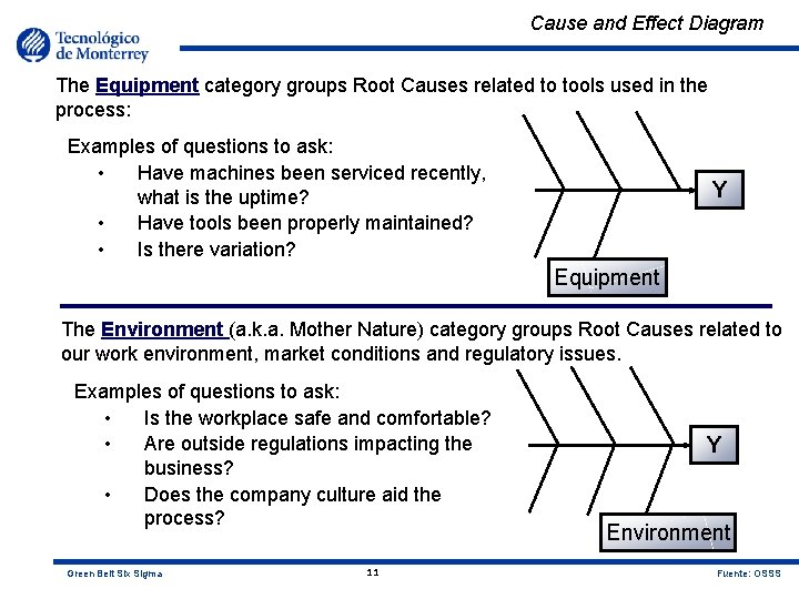
Cause and Effect Diagram The Measurement category groups Root Causes related to the measurement and measuring of a process activity or output: Examples of questions to ask: • Is there a metric issue? • Is there a valid measurement system? Is the data good enough? • Is data readily available? Measurement Y The People category groups Root Causes related to people, staffing and organizations: Examples of questions to ask: People • Are people trained, do they • • have the right skills? Is there person to person variation? Are people over-worked? Green Belt Six Sigma Y 9 Fuente: OSSS

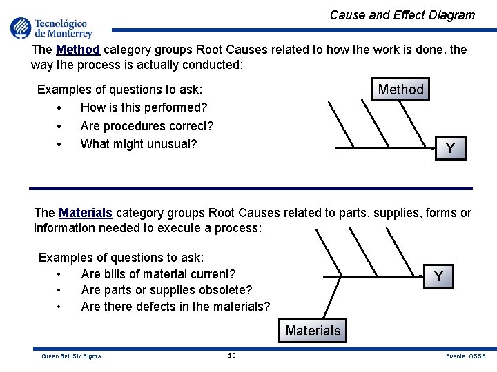
Cause and Effect Diagram The Method category groups Root Causes related to how the work is done, the way the process is actually conducted: Method Examples of questions to ask: • How is this performed? • Are procedures correct? • What might unusual? Y The Materials category groups Root Causes related to parts, supplies, forms or information needed to execute a process: Examples of questions to ask: • Are bills of material current? • Are parts or supplies obsolete? • Are there defects in the materials? Y Materials Green Belt Six Sigma 10 Fuente: OSSS

Cause and Effect Diagram The Equipment category groups Root Causes related to tools used in the process: Examples of questions to ask: • Have machines been serviced recently, what is the uptime? • Have tools been properly maintained? • Is there variation? Y Equipment The Environment (a. k. a. Mother Nature) category groups Root Causes related to our work environment, market conditions and regulatory issues. Examples of questions to ask: • Is the workplace safe and comfortable? • Are outside regulations impacting the business? • Does the company culture aid the process? Green Belt Six Sigma 11 Y Environment Fuente: OSSS

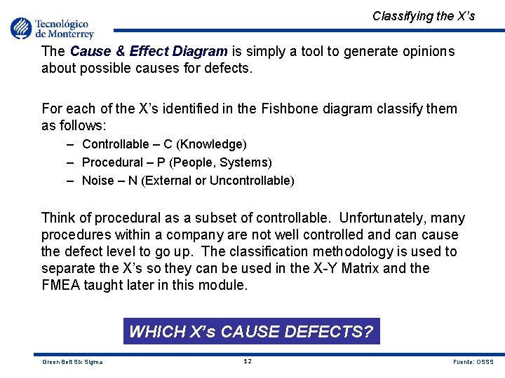
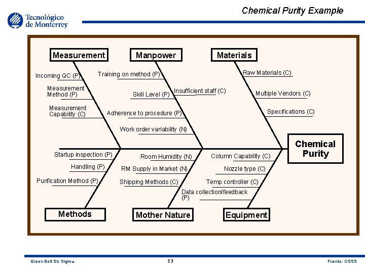
Classifying the X’s The Cause & Effect Diagram is simply a tool to generate opinions about possible causes for defects. For each of the X’s identified in the Fishbone diagram classify them as follows: – Controllable – C (Knowledge) – Procedural – P (People, Systems) – Noise – N (External or Uncontrollable) Think of procedural as a subset of controllable. Unfortunately, many procedures within a company are not well controlled and can cause the defect level to go up. The classification methodology is used to separate the X’s so they can be used in the X-Y Matrix and the FMEA taught later in this module. WHICH X’s CAUSE DEFECTS? Green Belt Six Sigma 12 Fuente: OSSS

Chemical Purity Example Measurement Incoming QC (P) Manpower Materials Raw Materials (C) Training on method (P) Measurement Method (P) Measurement Capability (C) Skill Level (P) Insufficient staff (C) Multiple Vendors (C) Specifications (C) Adherence to procedure (P) Work order variability (N) Startup inspection (P) Handling (P) Purification Method (P) Room Humidity (N) RM Supply in Market (N) Shipping Methods (C) Column Capability (C) Chemical Purity Nozzle type (C) Temp controller (C) Data collection/feedback (P) Methods Green Belt Six Sigma Mother Nature 13 Equipment Fuente: OSSS

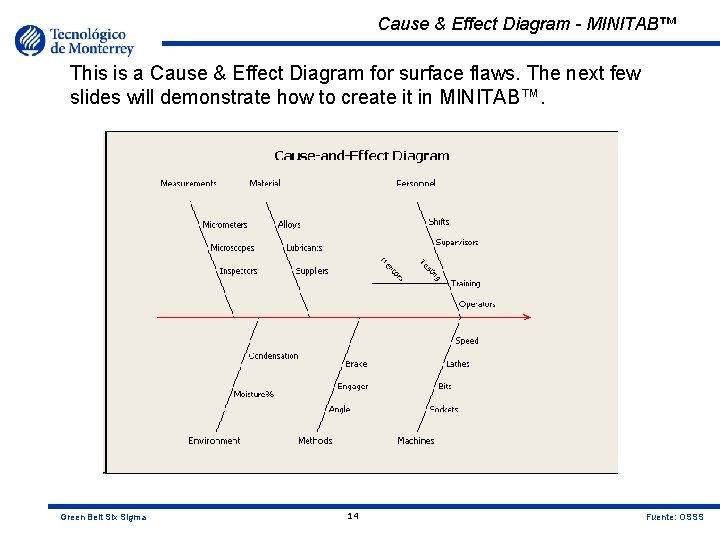
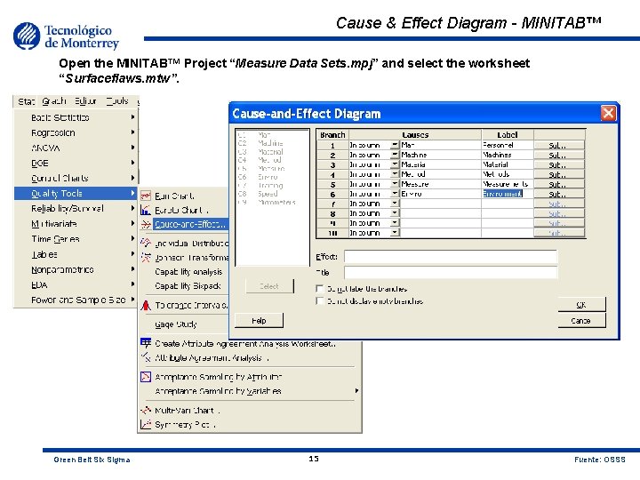
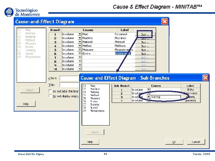
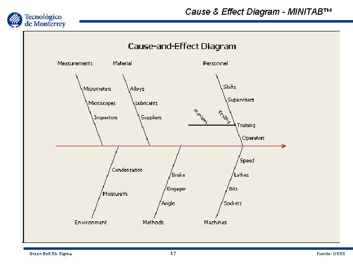
Cause & Effect Diagram - MINITAB™ This is a Cause & Effect Diagram for surface flaws. The next few slides will demonstrate how to create it in MINITAB™. Green Belt Six Sigma 14 Fuente: OSSS

Cause & Effect Diagram - MINITAB™ Open the MINITAB™ Project “Measure Data Sets. mpj” and select the worksheet “Surfaceflaws. mtw”. Green Belt Six Sigma 15 Fuente: OSSS

Cause & Effect Diagram - MINITAB™ Green Belt Six Sigma 16 Fuente: OSSS

Cause & Effect Diagram - MINITAB™ Green Belt Six Sigma 17 Fuente: OSSS

Cause & Effect Diagram Exercise objective: Create a Fishbone Diagram. 1. Retrieve the high level Process Map for your project and use it to complete a Fishbone, if possible include your project team. Don’t let the big one get away! Green Belt Six Sigma 18 Fuente: OSSS

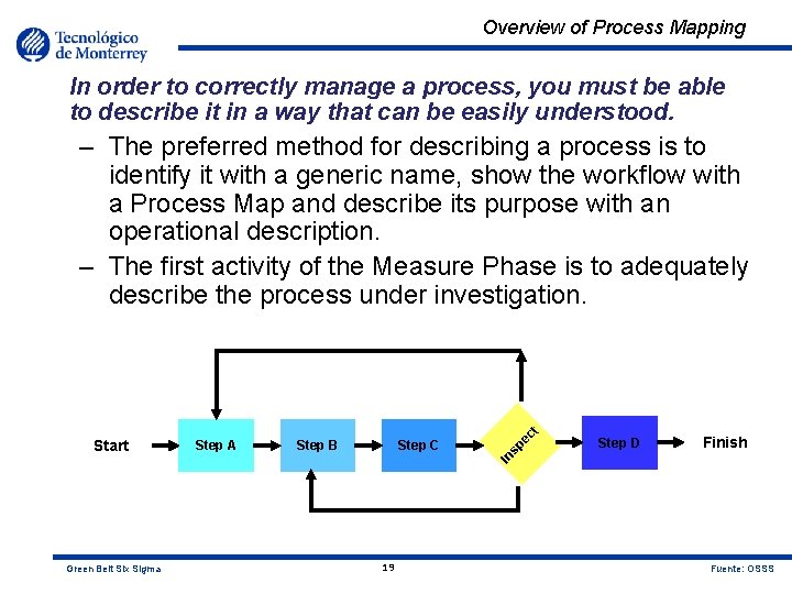
Overview of Process Mapping In order to correctly manage a process, you must be able to describe it in a way that can be easily understood. Step A Step B Step C Step D Finish In Start sp ec t – The preferred method for describing a process is to identify it with a generic name, show the workflow with a Process Map and describe its purpose with an operational description. – The first activity of the Measure Phase is to adequately describe the process under investigation. Green Belt Six Sigma 19 Fuente: OSSS

Information from Process Mapping By mapping processes we can identify many important characteristics and develop information for other analytical tools: 1. 2. 3. 4. 5. 6. Process inputs (X’s) Supplier requirements Process outputs (Y’s) Actual customer needs All value-added and non-value added process tasks and steps Data collection points • Cycle times • Defects • Inventory levels • Cost of poor quality, etc. 7. Decision points 8. Problems that have immediate fixes 9. Process control needs Green Belt Six Sigma 20 Fuente: OSSS

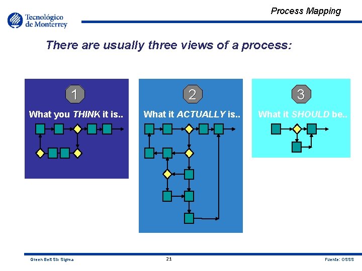
Process Mapping There are usually three views of a process: 1 2 3 What you THINK it is. . What it ACTUALLY is. . What it SHOULD be. . Green Belt Six Sigma 21 Fuente: OSSS

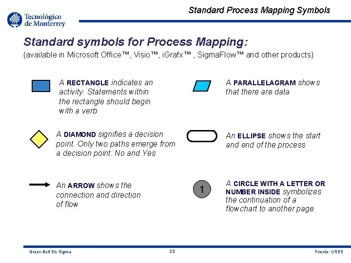
Standard Process Mapping Symbols Standard symbols for Process Mapping: (available in Microsoft Office™, Visio™, i. Grafx™ , Sigma. Flow™ and other products) A RECTANGLE indicates an activity. Statements within the rectangle should begin with a verb A PARALLELAGRAM shows that there are data A DIAMOND signifies a decision point. Only two paths emerge from a decision point: No and Yes An ARROW shows the connection and direction of flow Green Belt Six Sigma An ELLIPSE shows the start and end of the process 1 22 A CIRCLE WITH A LETTER OR NUMBER INSIDE symbolizes the continuation of a flowchart to another page Fuente: OSSS

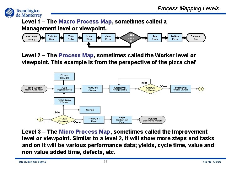
Process Mapping Levels Level 1 – The Macro Process Map, sometimes called a Management level or viewpoint. Customer Hungry Calls for Order Take Order Make Pizza Cook Pizza Corre ct Box Pizza Deliver Pizza Customer Eats Level 2 – The Process Map, sometimes called the Worker level or viewpoint. This example is from the perspective of the pizza chef Level 3 – The Micro Process Map, sometimes called the Improvement level or viewpoint. Similar to a level 2, it will show more steps and tasks and on it will be various performance data; yields, cycle time, value and non value added time, defects, etc. Green Belt Six Sigma 23 Fuente: OSSS

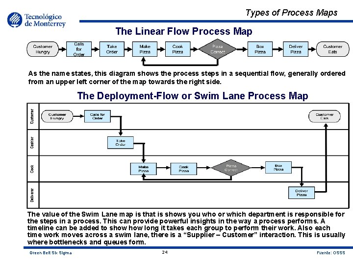
Types of Process Maps The Linear Flow Process Map As the name states, this diagram shows the process steps in a sequential flow, generally ordered from an upper left corner of the map towards the right side. The Deployment-Flow or Swim Lane Process Map The value of the Swim Lane map is that is shows you who or which department is responsible for the steps in a process. This can provide powerful insights in the way a process performs. A timeline can be added to show long it takes each group to perform their work. Also each time work moves across a swim lane, there is a “Supplier – Customer” interaction. This is usually where bottlenecks and queues form. Green Belt Six Sigma 24 Fuente: OSSS

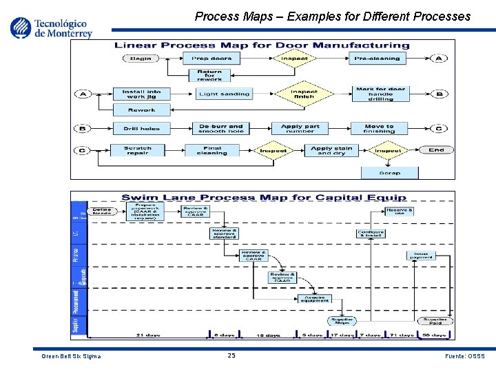
Process Maps – Examples for Different Processes Green Belt Six Sigma 25 Fuente: OSSS

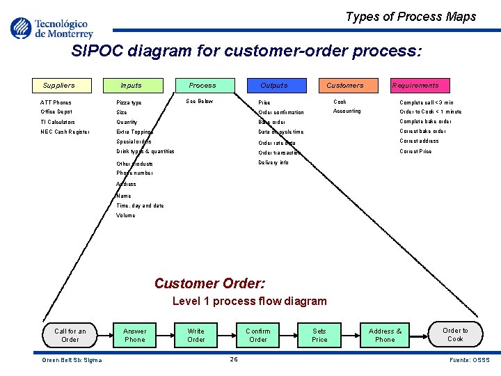
Types of Process Maps SIPOC diagram for customer-order process: Suppliers Inputs Process Outputs See Below Customers Requirements Price Cook Complete call < 3 min Size Order confirmation Accounting Order to Cook < 1 minute TI Calculators Quantity Bake order Complete bake order NEC Cash Register Extra Toppings Data on cycle time Correct bake order Special orders Order rate data Correct address Drink types & quantities Order transaction Correct Price Other products Delivery info ATT Phones Office Depot Pizza type Phone number Address Name Time, day and date Volume Customer Order: Level 1 process flow diagram Call for an Order Green Belt Six Sigma Answer Phone Write Order Confirm Order 26 Sets Price Address & Phone Order to Cook Fuente: OSSS

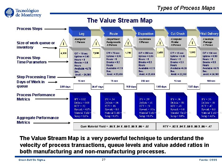
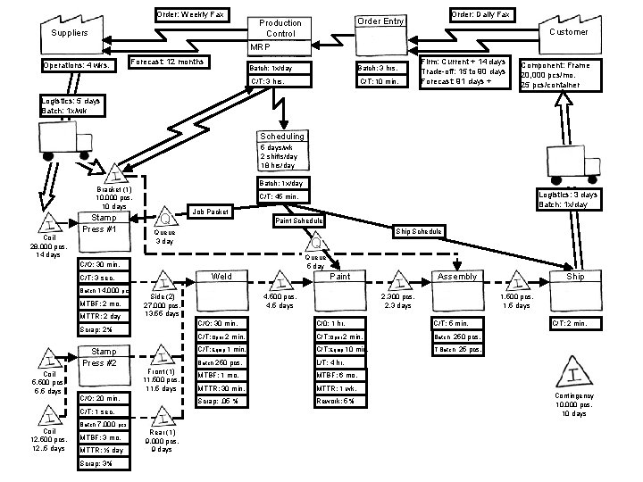
Types of Process Maps The Value Stream Map Process Steps Size of work queue or inventory Process Step Time Parameters Step Processing Time Days of Work in queue Process Performance Metrics Aggregate Performance Metrics The Value Stream Map is a very powerful technique to understand the velocity of process transactions, queue levels and value added ratios in both manufacturing and non-manufacturing processes. Green Belt Six Sigma 27 Fuente: OSSS

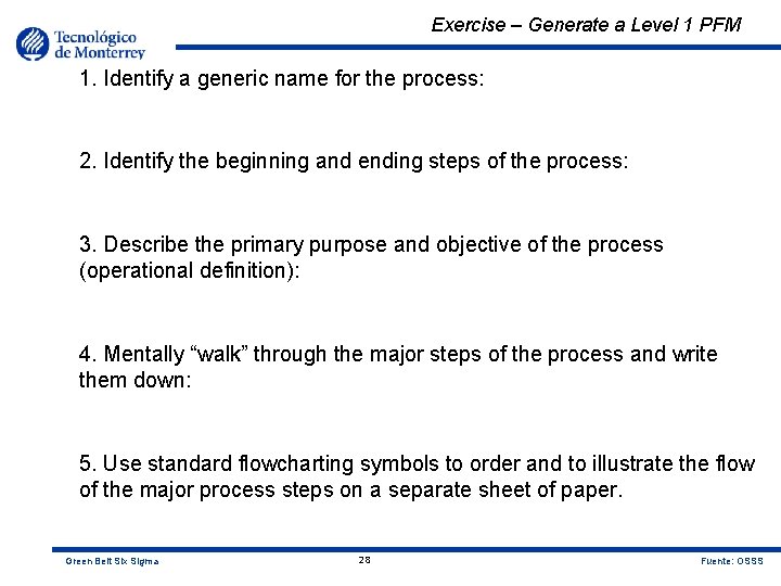
Exercise – Generate a Level 1 PFM 1. Identify a generic name for the process: 2. Identify the beginning and ending steps of the process: 3. Describe the primary purpose and objective of the process (operational definition): 4. Mentally “walk” through the major steps of the process and write them down: 5. Use standard flowcharting symbols to order and to illustrate the flow of the major process steps on a separate sheet of paper. Green Belt Six Sigma 28 Fuente: OSSS

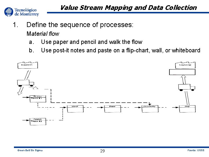
Value Stream Mapping and Data Collection 1. Define the sequence of processes: Material flow a. Use paper and pencil and walk the flow b. Use post-it notes and paste on a flip-chart, wall, or whiteboard Green Belt Six Sigma 29 Fuente: OSSS

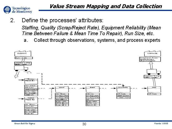
Value Stream Mapping and Data Collection 2. Define the processes’ attributes: Staffing, Quality (Scrap/Reject Rate), Equipment Reliability (Mean Time Between Failure & Mean Time To Repair), Run Size, etc. a. Collect through observations, systems, and process experts Green Belt Six Sigma 30 Fuente: OSSS

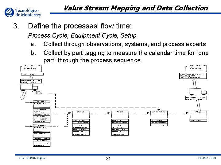
Value Stream Mapping and Data Collection 3. Define the processes’ flow time: Process Cycle, Equipment Cycle, Setup a. Collect through observations, systems, and process experts b. Collect by part tagging to measure the calendar time for “one part” through the process sequence Green Belt Six Sigma 31 Fuente: OSSS

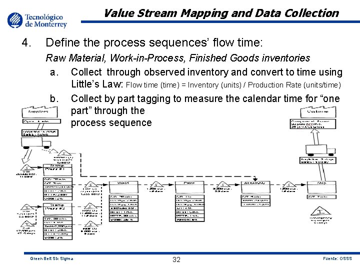
Value Stream Mapping and Data Collection 4. Define the process sequences’ flow time: Raw Material, Work-in-Process, Finished Goods inventories a. Collect through observed inventory and convert to time using Little’s Law: Flow time (time) = Inventory (units) / Production Rate (units/time) b. Collect by part tagging to measure the calendar time for “one part” through the process sequence Green Belt Six Sigma 32 Fuente: OSSS

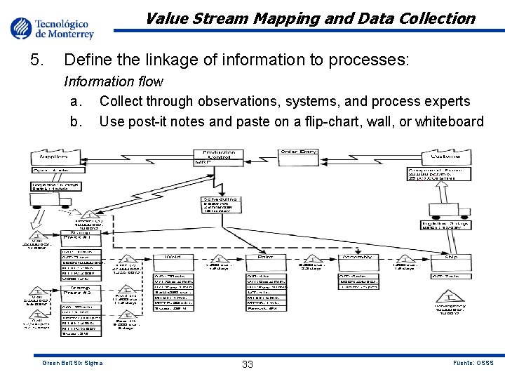
Value Stream Mapping and Data Collection 5. Define the linkage of information to processes: Information flow a. Collect through observations, systems, and process experts b. Use post-it notes and paste on a flip-chart, wall, or whiteboard Green Belt Six Sigma 33 Fuente: OSSS

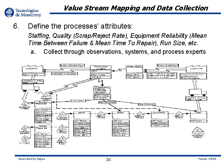
Value Stream Mapping and Data Collection 6. Define the processes’ attributes: Staffing, Quality (Scrap/Reject Rate), Equipment Reliability (Mean Time Between Failure & Mean Time To Repair), Run Size, etc. a. Collect through observations, systems, and process experts Green Belt Six Sigma 34 Fuente: OSSS

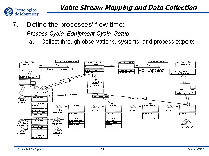
Value Stream Mapping and Data Collection 7. Define the processes’ flow time: Process Cycle, Equipment Cycle, Setup a. Collect through observations, systems, and process experts Green Belt Six Sigma 35 Fuente: OSSS

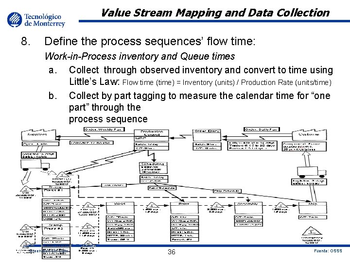
Value Stream Mapping and Data Collection 8. Define the process sequences’ flow time: Work-in-Process inventory and Queue times a. Collect through observed inventory and convert to time using Little’s Law: Flow time (time) = Inventory (units) / Production Rate (units/time) b. Collect by part tagging to measure the calendar time for “one part” through the process sequence Green Belt Six Sigma 36 Fuente: OSSS

Order: Weekly Fax Suppliers Operations: 4 wks. Forecast: 12 months Production Control MRP Order Entry Batch: 1 x/day Batch: 3 hrs. C/T: 10 min. Order: Daily Fax Customer Firm: Current + 14 days Trade-off: 15 to 90 days Forecast: 91 days + Component: Frame 20, 000 pcs/mo. 25 pcs/container Logistics: 5 days Batch: 1 x/wk Scheduling 5 days/wk 2 shifts/day 18 hrs/day Batch: 1 x/day Bracket (1) 10, 000 pcs. 10 days Stamp Press #1 Coil 28, 000 pcs. 14 days Q Job Packet Paint Schedule Queue 3 day Q Weld C/T: 3 sec. MTBF: 2 mo. MTTR: 2 day Coil 5, 500 pcs. 5. 5 days Front (1) 11, 500 pcs. 11. 5 days C/O: 20 min. Paint 4, 500 pcs. 4. 5 days Side (2) 27, 000 pcs. 13. 55 days Scrap: 2% Stamp Press #2 Batch: 7, 000 pcs. MTBF: 3 mo. MTTR: ½ day Green Belt Six 3% Sigma Scrap: Assembly 2, 300 pcs. 2. 3 days Ship 1, 500 pcs. 1. 5 days C/O: 30 min. C/0: 1 hr. C/T: 5 min. C/T: Oper 2 min. Batch: 250 pcs. C/T: Equip 1 min. C/T: Equip 10 min. T Batch: 25 pcs. Batch: 250 pcs. L/T: 4 hr. MTBF: 1 mo. MTBF: 6 mo. MTTR: 30 min. MTTR: 1 wk. Scrap: . 05 % Rework: 5% C/T: 1 sec. Coil 12, 500 pcs. 12. . 5 days Ship Schedule Queue 5 day C/O: 30 min. Batch: 14, 000 pcs. Logistics: 3 days Batch: 1 x/day C/T: 45 min. C/T: 2 min. Contingency 10, 000 pcs. 10 days Rear (1) 9, 000 pcs. 9 days 37 Fuente: OSSS

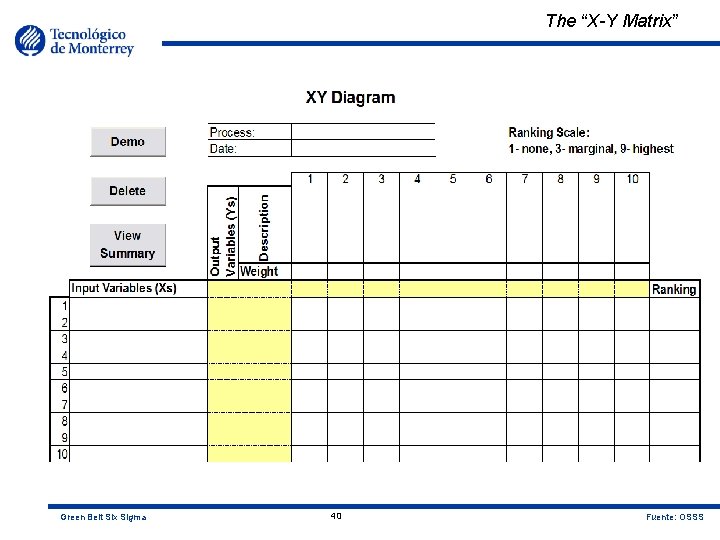
Definition of X-Y Matrix • The X-Y Matrix is: – A tool used to identify/collate potential X’s and assess their relative impact on multiple Y’s (include all Y’s that are customer focused) – Based on the team’s collective “opinions” – Created for every project – Never completed – Updated whenever a parameter is changed • To summarize, the X-Y is a team-based prioritization tool for the potential X’s. • WARNING! This is not real data, this is organized brainstorming!! At the conclusion of the project you may realize that the things you thought were critical are in fact not as important as was believed. Green Belt Six Sigma 38 Fuente: OSSS

The Vital Few A Belt does not just discover which X’s are important in a process (the vital few). – The team considers all possible X’s that can contribute or cause the problem observed. – The team uses 3 primary sources of X identification: • Process Mapping • Fishbone Analysis • Basic Data Analysis – Graphical and Statistical – A List of X’s is established and compiled. – The team then prioritizes which X’s it will explore first, and eliminates the “obvious” low impact X’s from further consideration. The X-Y Matrix is this Prioritization Tool! Green Belt Six Sigma 39 Fuente: OSSS

The “X-Y Matrix” Green Belt Six Sigma 40 Fuente: OSSS

Using the Classified X’s • Breakthrough requires dealing primarily with controllable X’s impacting the “Y”. • Use the controllable X’s from the Fishbone analysis to include in the X-Y Matrix. • The goal is to isolate the vital few X’s from the trivial many X’s. • Procedures and Noise X’s will be used in the FMEA at the end of this module. However: – All procedures must be in total compliance. • This may require some type of effectiveness measure. • This could reduce or eliminate some of the defects currently seen in the process (allowing focus on controllable X’s). – Noise type inputs increase risk of defects under current technology of operation and therefore: • Increase RPN on the FMEA document from an input. • Help identify areas needing investment for a justified ROI. *Risk Priority Number Green Belt Six Sigma 41 Fuente: OSSS

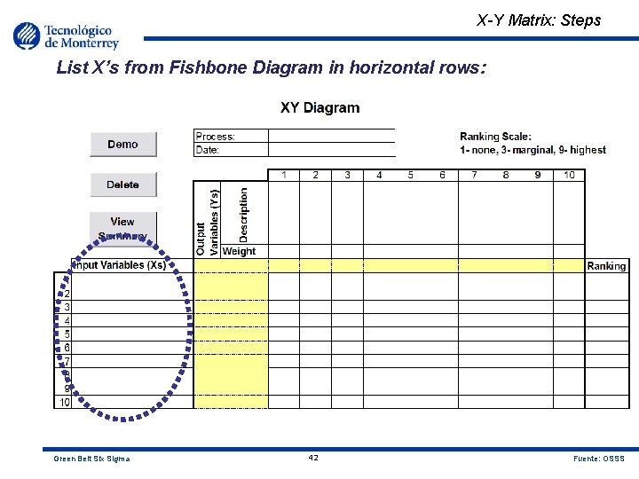
X-Y Matrix: Steps List X’s from Fishbone Diagram in horizontal rows: Green Belt Six Sigma 42 Fuente: OSSS

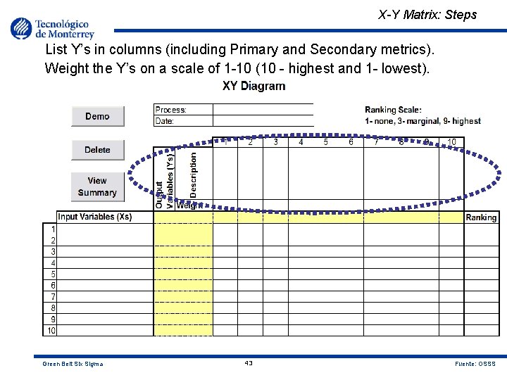
X-Y Matrix: Steps List Y’s in columns (including Primary and Secondary metrics). Weight the Y’s on a scale of 1 -10 (10 - highest and 1 - lowest). Green Belt Six Sigma 43 Fuente: OSSS

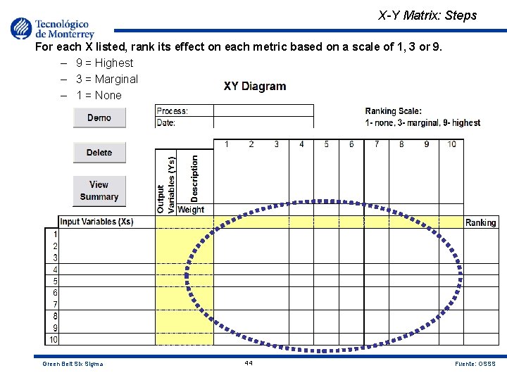
X-Y Matrix: Steps For each X listed, rank its effect on each metric based on a scale of 1, 3 or 9. – 9 = Highest – 3 = Marginal – 1 = None Green Belt Six Sigma 44 Fuente: OSSS

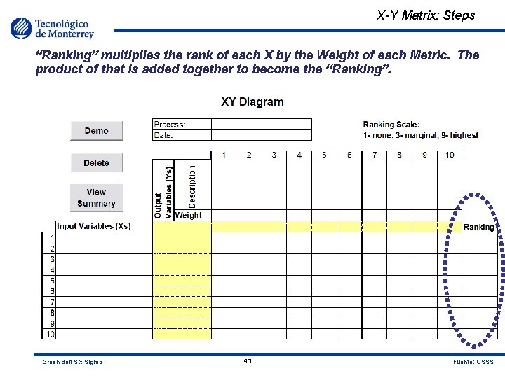
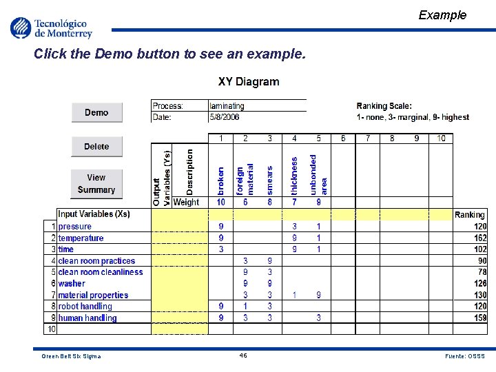
X-Y Matrix: Steps “Ranking” multiplies the rank of each X by the Weight of each Metric. The product of that is added together to become the “Ranking”. Green Belt Six Sigma 45 Fuente: OSSS

Example Click the Demo button to see an example. Green Belt Six Sigma 46 Fuente: OSSS

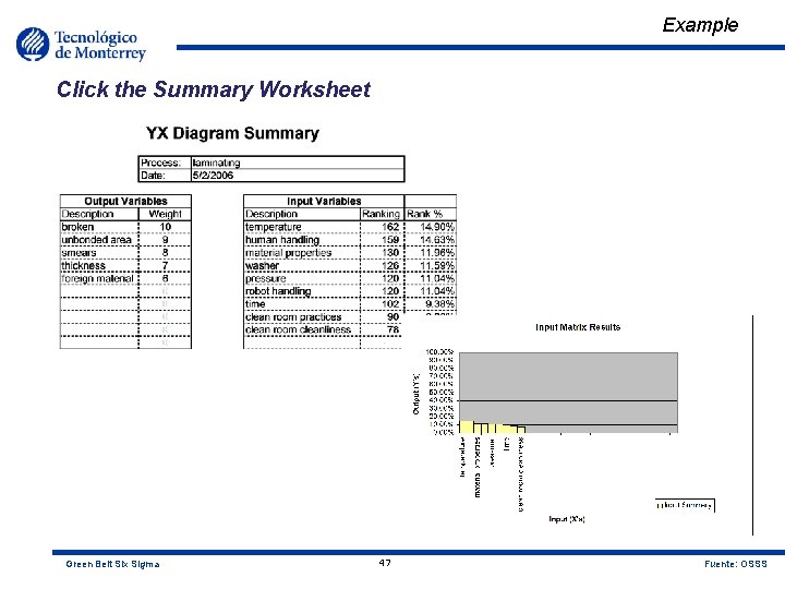
Example Click the Summary Worksheet Green Belt Six Sigma 47 Fuente: OSSS

Fishbone Diagram Exercise objective: Create an X-Y Matrix using the information from the Fishbone analysis. 1. Using the Fishbone Diagram created earlier, create an X-Y Matrix. 2. Present results to your mentor. Green Belt Six Sigma 48 Fuente: OSSS

Summary At this point, you should be able to: • Create a high-level Process Map • Create a Fishbone Diagram • Create an X-Y Matrix • Describe the purpose of each tool and when it should be used Green Belt Six Sigma 49 Fuente: OSSS

Measure Phase Six Sigma Statistics

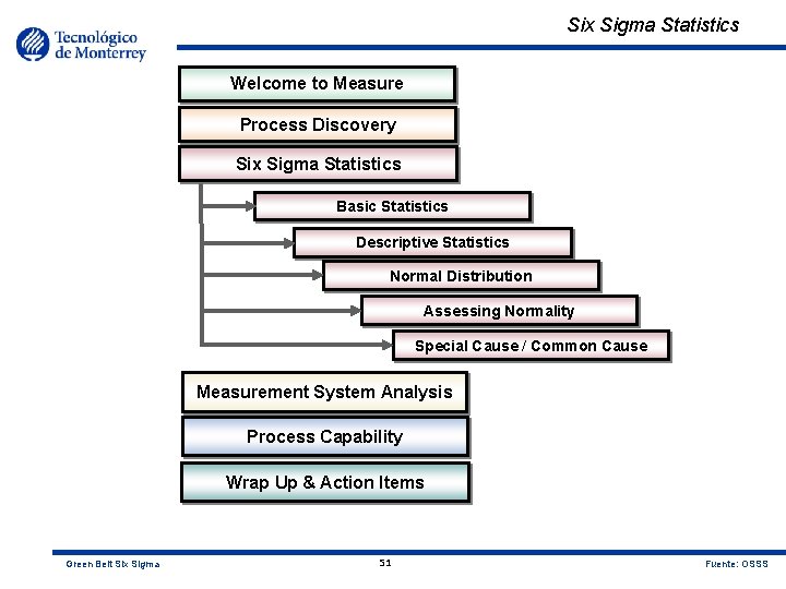
Six Sigma Statistics Welcome to Measure Process Discovery Six Sigma Statistics Basic Statistics Descriptive Statistics Normal Distribution Assessing Normality Special Cause / Common Cause Measurement System Analysis Process Capability Wrap Up & Action Items Green Belt Six Sigma 51 Fuente: OSSS

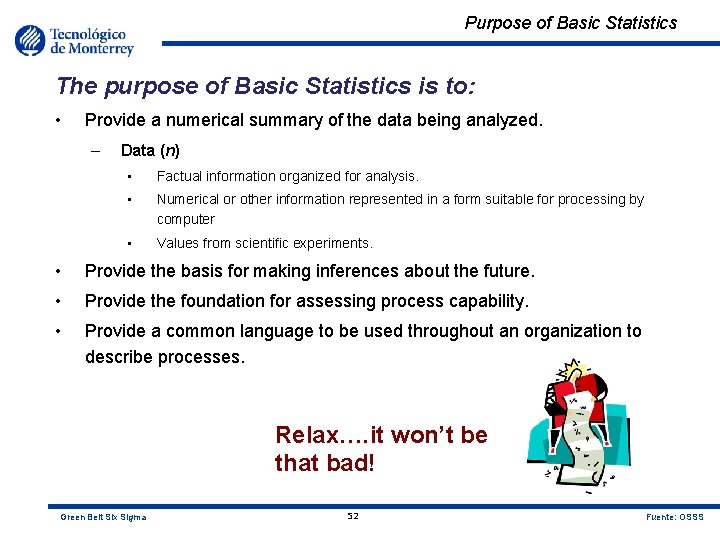
Purpose of Basic Statistics The purpose of Basic Statistics is to: • Provide a numerical summary of the data being analyzed. – Data (n) • Factual information organized for analysis. • Numerical or other information represented in a form suitable for processing by computer • Values from scientific experiments. • Provide the basis for making inferences about the future. • Provide the foundation for assessing process capability. • Provide a common language to be used throughout an organization to describe processes. Relax…. it won’t be that bad! Green Belt Six Sigma 52 Fuente: OSSS

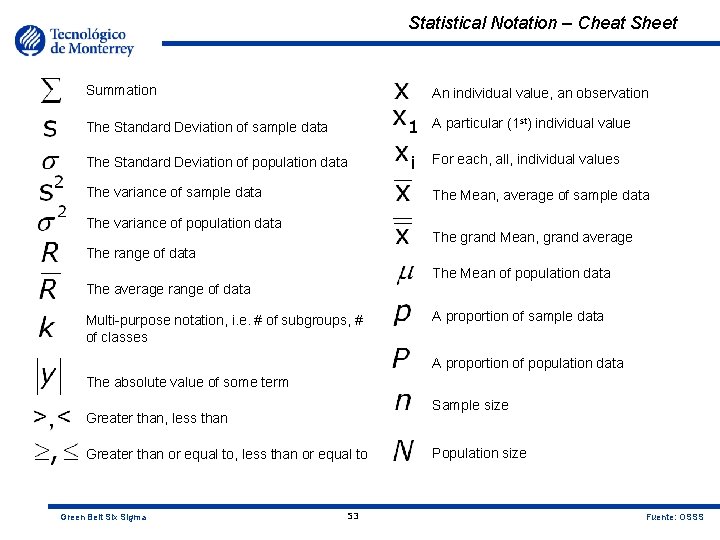
Statistical Notation – Cheat Sheet Summation An individual value, an observation The Standard Deviation of sample data A particular (1 st) individual value The Standard Deviation of population data For each, all, individual values The variance of sample data The Mean, average of sample data The variance of population data The grand Mean, grand average The range of data The Mean of population data The average range of data Multi-purpose notation, i. e. # of subgroups, # of classes A proportion of sample data A proportion of population data The absolute value of some term Sample size Greater than, less than Greater than or equal to, less than or equal to Green Belt Six Sigma 53 Population size Fuente: OSSS

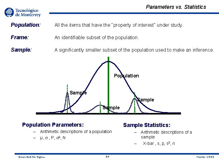
Parameters vs. Statistics Population: All the items that have the “property of interest” under study. Frame: An identifiable subset of the population. Sample: A significantly smaller subset of the population used to make an inference. Population Sample Population Parameters: Sample Statistics: – Arithmetic descriptions of a population – µ, , P, 2, N Green Belt Six Sigma 54 – Arithmetic descriptions of a sample – X-bar , s, p, s 2, n Fuente: OSSS

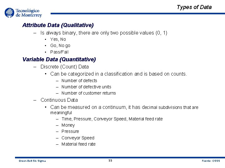
Types of Data Attribute Data (Qualitative) – Is always binary, there are only two possible values (0, 1) • Yes, No • Go, No go • Pass/Fail Variable Data (Quantitative) – Discrete (Count) Data • Can be categorized in a classification and is based on counts. – Number of defects – Number of defective units – Number of customer returns – Continuous Data • Can be measured on a continuum, it has decimal subdivisions that are meaningful – Time, Pressure, Conveyor Speed, Material feed rate – Money – Pressure – Conveyor Speed – Material feed rate Green Belt Six Sigma 55 Fuente: OSSS

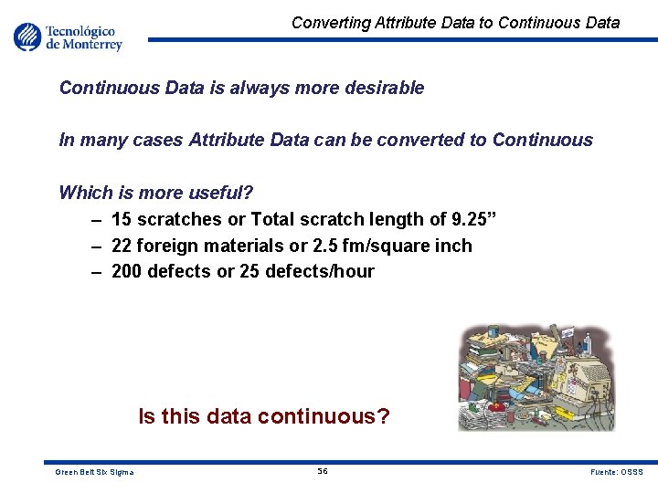
Converting Attribute Data to Continuous Data is always more desirable In many cases Attribute Data can be converted to Continuous Which is more useful? – 15 scratches or Total scratch length of 9. 25” – 22 foreign materials or 2. 5 fm/square inch – 200 defects or 25 defects/hour Is this data continuous? Green Belt Six Sigma 56 Fuente: OSSS

Descriptive Statistics Measures of Location (central tendency) – Mean – Median – Mode Measures of Variation (dispersion) – – Range Interquartile Range Standard deviation Variance Green Belt Six Sigma 57 Fuente: OSSS

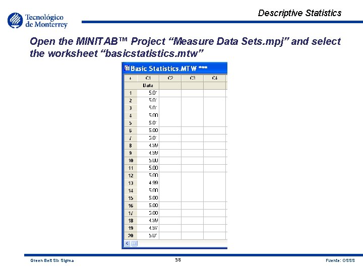
Descriptive Statistics Open the MINITAB™ Project “Measure Data Sets. mpj” and select the worksheet “basicstatistics. mtw” Green Belt Six Sigma 58 Fuente: OSSS

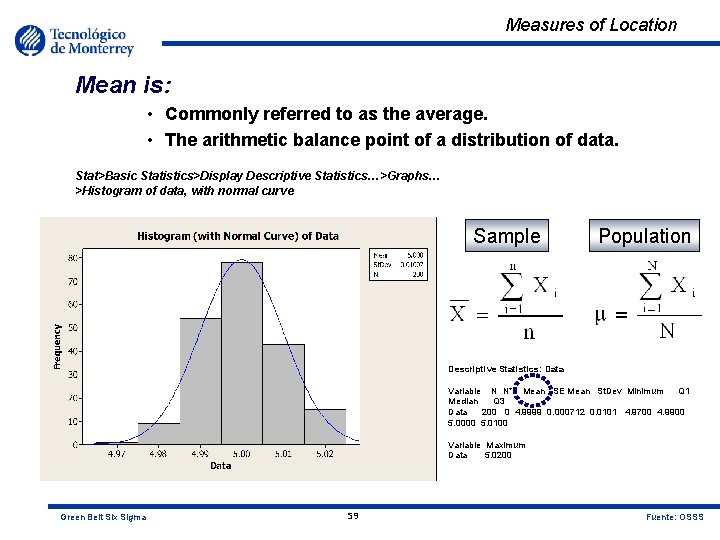
Measures of Location Mean is: • Commonly referred to as the average. • The arithmetic balance point of a distribution of data. Stat>Basic Statistics>Display Descriptive Statistics…>Graphs… >Histogram of data, with normal curve Sample Population Descriptive Statistics: Data Variable N N* Mean SE Mean St. Dev Minimum Q 1 Median Q 3 Data 200 0 4. 9999 0. 000712 0. 0101 4. 9700 4. 9900 5. 0000 5. 0100 Variable Maximum Data 5. 0200 Green Belt Six Sigma 59 Fuente: OSSS

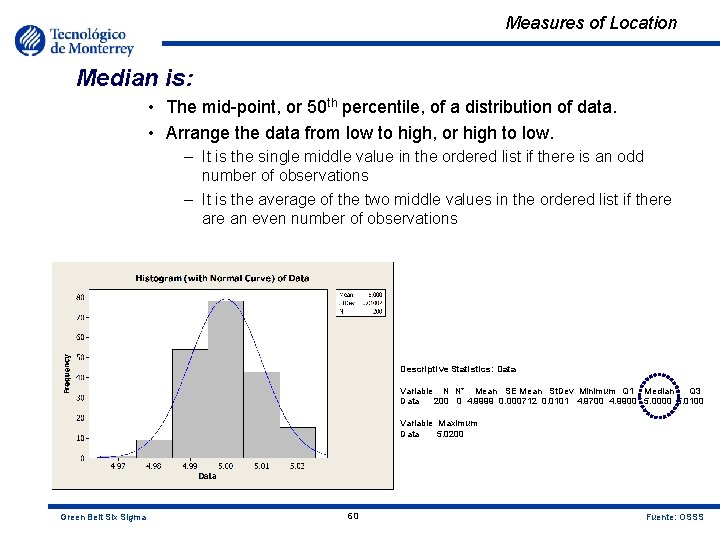
Measures of Location Median is: • The mid-point, or 50 th percentile, of a distribution of data. • Arrange the data from low to high, or high to low. – It is the single middle value in the ordered list if there is an odd number of observations – It is the average of the two middle values in the ordered list if there an even number of observations Descriptive Statistics: Data Variable N N* Mean SE Mean St. Dev Minimum Q 1 Median Q 3 Data 200 0 4. 9999 0. 000712 0. 0101 4. 9700 4. 9900 5. 0000 5. 0100 Variable Maximum Data 5. 0200 Green Belt Six Sigma 60 Fuente: OSSS

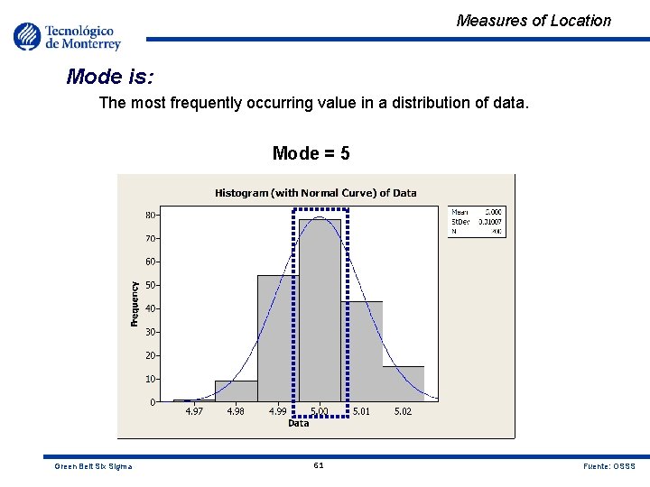
Measures of Location Mode is: The most frequently occurring value in a distribution of data. Mode = 5 Green Belt Six Sigma 61 Fuente: OSSS

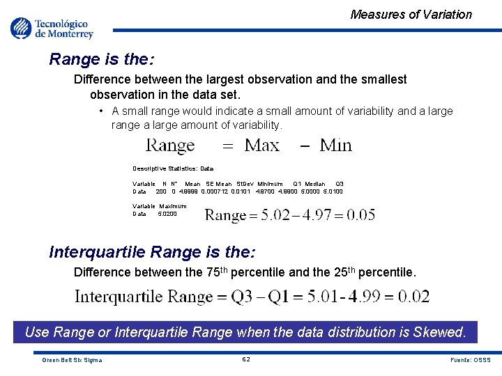
Measures of Variation Range is the: Difference between the largest observation and the smallest observation in the data set. • A small range would indicate a small amount of variability and a large range a large amount of variability. Descriptive Statistics: Data Variable N N* Mean SE Mean St. Dev Minimum Q 1 Median Q 3 Data 200 0 4. 9999 0. 000712 0. 0101 4. 9700 4. 9900 5. 0000 5. 0100 Variable Maximum Data 5. 0200 Interquartile Range is the: Difference between the 75 th percentile and the 25 th percentile. Use Range or Interquartile Range when the data distribution is Skewed. Green Belt Six Sigma 62 Fuente: OSSS

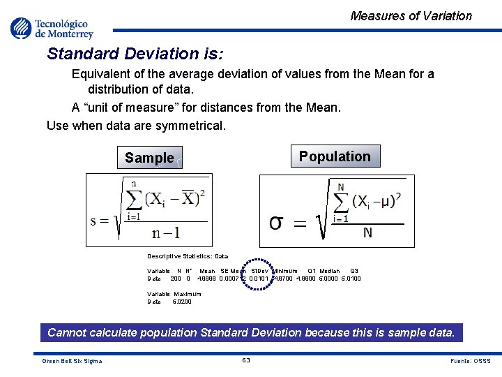
Measures of Variation Standard Deviation is: Equivalent of the average deviation of values from the Mean for a distribution of data. A “unit of measure” for distances from the Mean. Use when data are symmetrical. Population Sample Descriptive Statistics: Data Variable N N* Mean SE Mean St. Dev Minimum Q 1 Median Q 3 Data 200 0 4. 9999 0. 000712 0. 0101 4. 9700 4. 9900 5. 0000 5. 0100 Variable Maximum Data 5. 0200 Cannot calculate population Standard Deviation because this is sample data. Green Belt Six Sigma 63 Fuente: OSSS

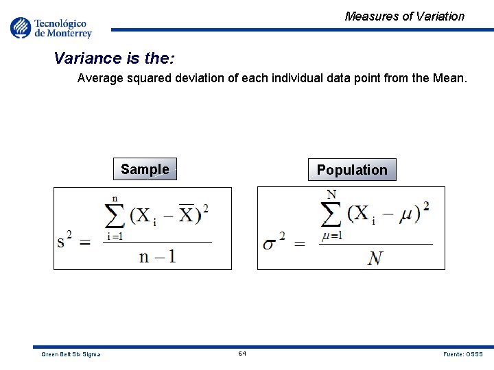
Measures of Variation Variance is the: Average squared deviation of each individual data point from the Mean. Sample Green Belt Six Sigma Population 64 Fuente: OSSS

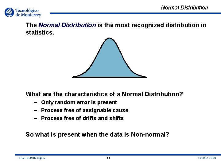
Normal Distribution The Normal Distribution is the most recognized distribution in statistics. What are the characteristics of a Normal Distribution? – Only random error is present – Process free of assignable cause – Process free of drifts and shifts So what is present when the data is Non-normal? Green Belt Six Sigma 65 Fuente: OSSS

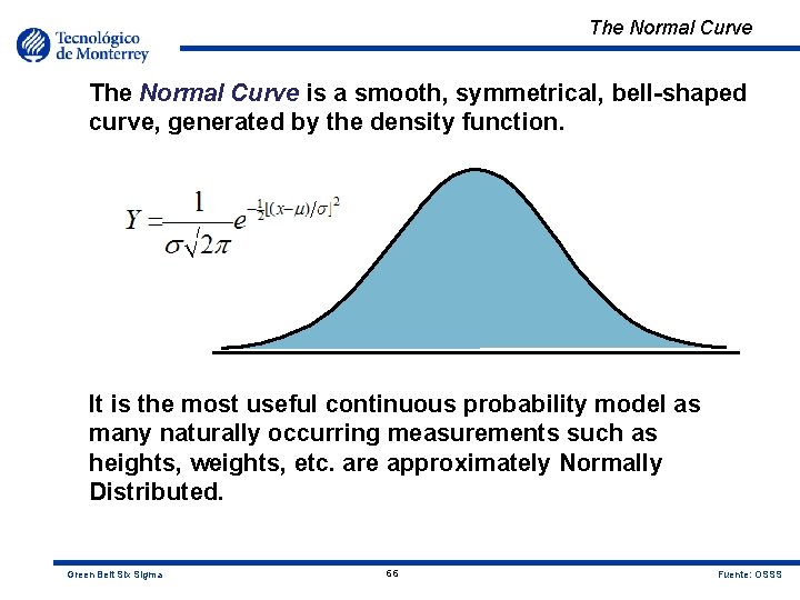
The Normal Curve is a smooth, symmetrical, bell-shaped curve, generated by the density function. It is the most useful continuous probability model as many naturally occurring measurements such as heights, weights, etc. are approximately Normally Distributed. Green Belt Six Sigma 66 Fuente: OSSS

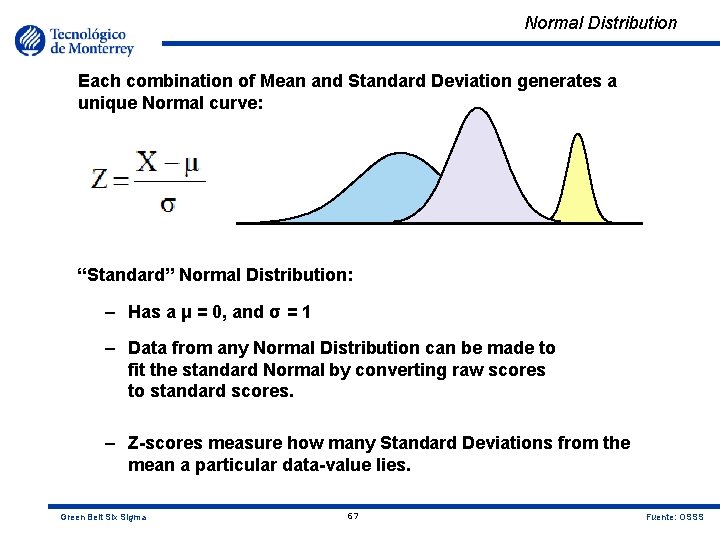
Normal Distribution Each combination of Mean and Standard Deviation generates a unique Normal curve: “Standard” Normal Distribution: – Has a μ = 0, and σ = 1 – Data from any Normal Distribution can be made to fit the standard Normal by converting raw scores to standard scores. – Z-scores measure how many Standard Deviations from the mean a particular data-value lies. Green Belt Six Sigma 67 Fuente: OSSS

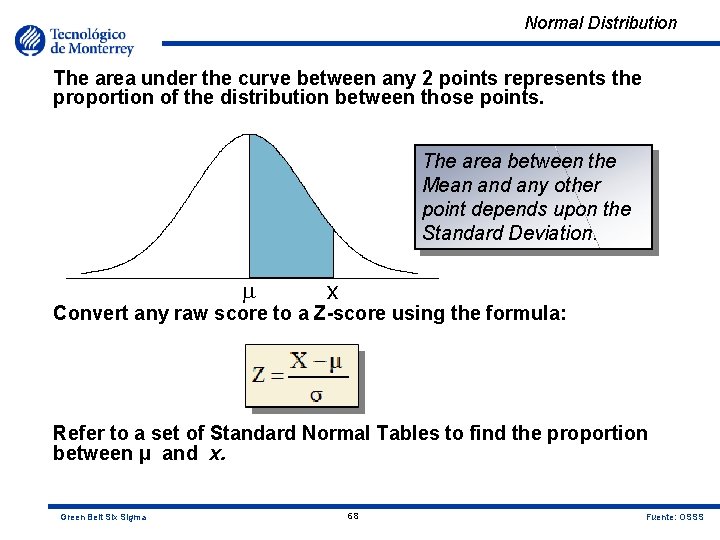
Normal Distribution The area under the curve between any 2 points represents the proportion of the distribution between those points. The area between the Mean and any other point depends upon the Standard Deviation. m x Convert any raw score to a Z-score using the formula: Refer to a set of Standard Normal Tables to find the proportion between μ and x. Green Belt Six Sigma 68 Fuente: OSSS

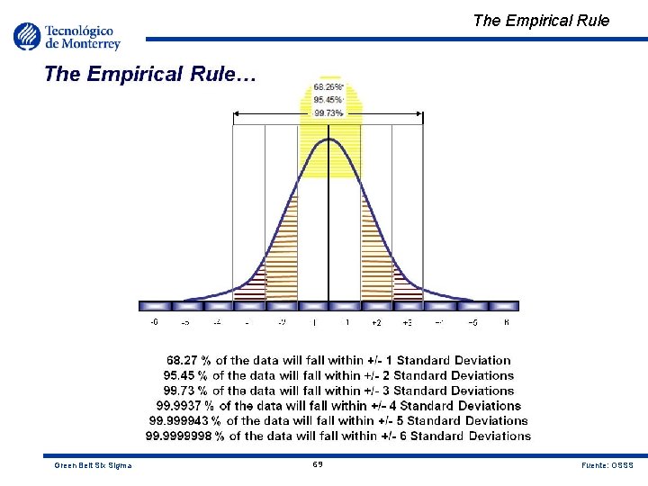
The Empirical Rule… -6 Green Belt Six Sigma -5 -4 -3 -2 -1 69 +1 +2 +3 +4 +5 +6 Fuente: OSSS

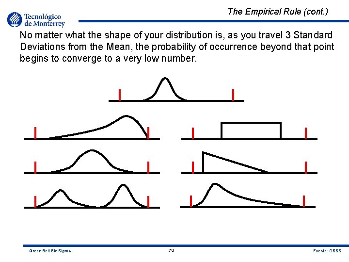
The Empirical Rule (cont. ) No matter what the shape of your distribution is, as you travel 3 Standard Deviations from the Mean, the probability of occurrence beyond that point begins to converge to a very low number. Green Belt Six Sigma 70 Fuente: OSSS

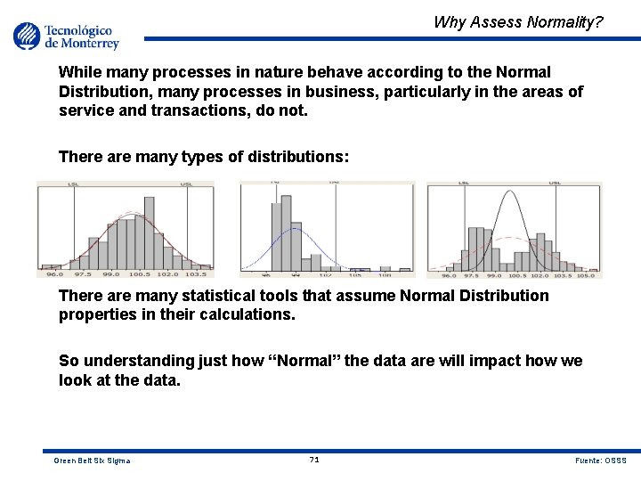
Why Assess Normality? While many processes in nature behave according to the Normal Distribution, many processes in business, particularly in the areas of service and transactions, do not. There are many types of distributions: There are many statistical tools that assume Normal Distribution properties in their calculations. So understanding just how “Normal” the data are will impact how we look at the data. Green Belt Six Sigma 71 Fuente: OSSS

Tools for Assessing Normality The shape of any Normal curve can be calculated based on the Normal Probability density function. Tests for Normality basically compare the shape of the calculated curve to the actual distribution of your data points. For the purposes of this training, we will focus on 2 ways in MINITAB™ to assess Normality: – The Anderson-Darling test – Normal probability test Watch that curve! Green Belt Six Sigma 72 Fuente: OSSS

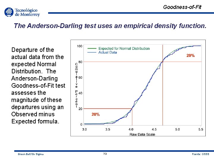
Goodness-of-Fit The Anderson-Darling test uses an empirical density function. Departure of the actual data from the expected Normal Distribution. The Anderson-Darling Goodness-of-Fit test assesses the magnitude of these departures using an Observed minus Expected formula. Green Belt Six Sigma 73 Fuente: OSSS

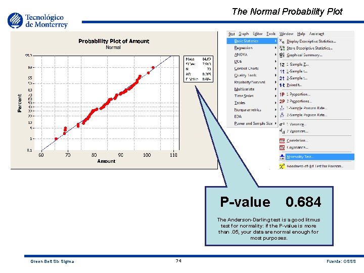
The Normal Probability Plot P-value 0. 684 The Anderson-Darling test is a good litmus test for normality: if the P-value is more than. 05, your data are normal enough for most purposes. Green Belt Six Sigma 74 Fuente: OSSS

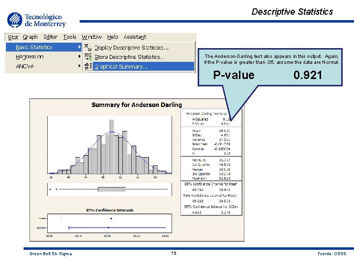
Descriptive Statistics The Anderson-Darling test also appears in this output. Again, if the P-value is greater than. 05, assume the data are Normal. P-value Green Belt Six Sigma 75 0. 921 Fuente: OSSS

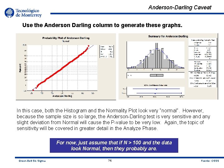
Anderson-Darling Caveat Use the Anderson Darling column to generate these graphs. In this case, both the Histogram and the Normality Plot look very “normal”. However, because the sample size is so large, the Anderson-Darling test is very sensitive and any slight deviation from Normal will cause the P-value to be very low. Again, the topic of sensitivity will be covered in greater detail in the Analyze Phase. For now, just assume that if N > 100 and the data look Normal, then they probably are. Green Belt Six Sigma 76 Fuente: OSSS

If the Data Are Not Normal, Don’t Panic! • Normal Data are not common in the transactional world. • There are lots of meaningful statistical tools you can use to analyze your data (more on that later). • It just means you may have to think about your data in a slightly different way. Don’t touch that button! Green Belt Six Sigma 77 Fuente: OSSS

Normality Exercise objective: To demonstrate how to test for Normality. 1. Generate Normal Probability Plots and the graphical summary using the “Descriptive Statistics. MTW” file. 2. Use only the columns Dist A and Dist D. 3. Answer the following quiz questions based on your analysis of this data set. Green Belt Six Sigma 78 Fuente: OSSS

Isolating Special Causes from Common Causes Special Cause: Variation is caused by known factors that result in a non-random distribution of output. Also referred to as “Assignable Cause”. Common Cause: Variation caused by unknown factors resulting in a steady but random distribution of output around the average of the data. It is the variation left over after Special Cause variation has been removed and typically (not always) follows a Normal Distribution. If we know that the basic structure of the data should follow a Normal Distribution, but plots from our data shows otherwise; we know the data contain Special Causes = Opportunity Green Belt Six Sigma 79 Fuente: OSSS

Summary At this point, you should be able to: • Explain the various statistics used to express location and spread of data • Describe characteristics of a Normal Distribution • Explain Special Cause variation Green Belt Six Sigma 80 Fuente: OSSS

Measure Phase Measurement System Analysis

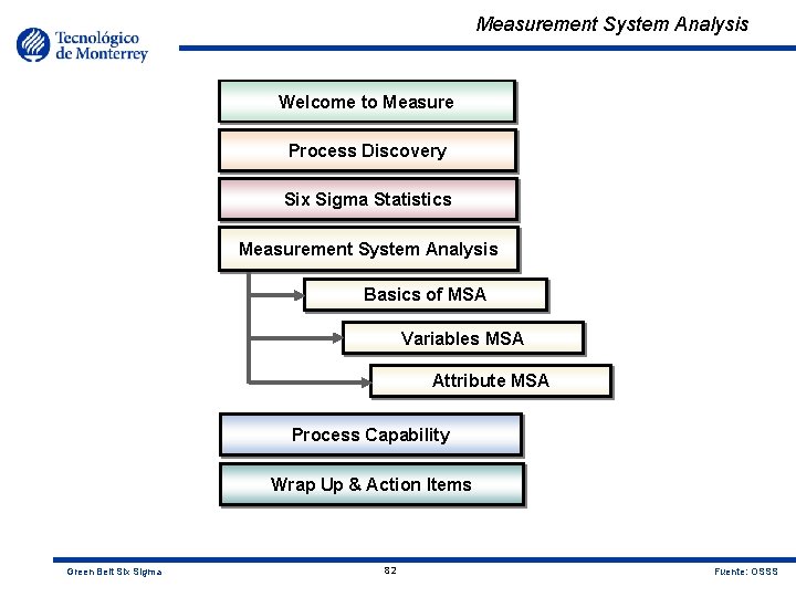
Measurement System Analysis Welcome to Measure Process Discovery Six Sigma Statistics Measurement System Analysis Basics of MSA Variables MSA Attribute MSA Process Capability Wrap Up & Action Items Green Belt Six Sigma 82 Fuente: OSSS

Introduction to MSA So far we have learned that the heart and soul of Six Sigma is that it is a data-driven methodology. – How do you know that the data you have used is accurate and precise? – How do know if a measurement is a repeatable and reproducible? How good are these? Measurement System Analysis or MSA Green Belt Six Sigma 83 Fuente: OSSS

Measurement System Analysis MSA is a mathematical procedure to quantify variation introduced to a process or product by the act of measuring. Reference Item to be Measured Measurement Operator Measurement Process Equipment Procedure Environment The item to be measured can be a physical part, document or a scenario for customer service. Operator can refer to a person or can be different instruments measuring the same products. Reference is a standard that is used to calibrate the equipment. Procedure is the method used to perform the test. Equipment is the device used to measure the product. Environment is the surroundings where the measures are performed. Green Belt Six Sigma 84 Fuente: OSSS

Measurement Purpose In order to be worth collecting, measurements must provide value that is, they must provide us with information and ultimately, knowledge The question… What do I need to know? …must be answered before we begin to consider issues of measurements, metrics, statistics, or data collection systems Too often, organizations build complex data collection and information management systems without truly understanding how the data collected and metrics calculated actually benefit the organization. Green Belt Six Sigma 85 Fuente: OSSS

Purpose The purpose of MSA is to assess the error due to measurement systems. The error can be partitioned into specific sources: – Precision • Repeatability - within an operator or piece of equipment • Reproducibility - operator to operator or attribute gage to attribute gage – Accuracy • Stability - accuracy over time • Linearity- accuracy throughout the measurement range • Resolution • Bias – Off-set from true value – Constant Bias – Variable Bias – typically seen with electronic equipment, amount of Bias changes with setting levels Green Belt Six Sigma 86 Fuente: OSSS

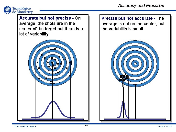
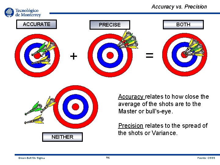
Accuracy and Precision Accurate but not precise - On average, the shots are in the center of the target but there is a lot of variability Green Belt Six Sigma Precise but not accurate - The average is not on the center, but the variability is small 87 Fuente: OSSS

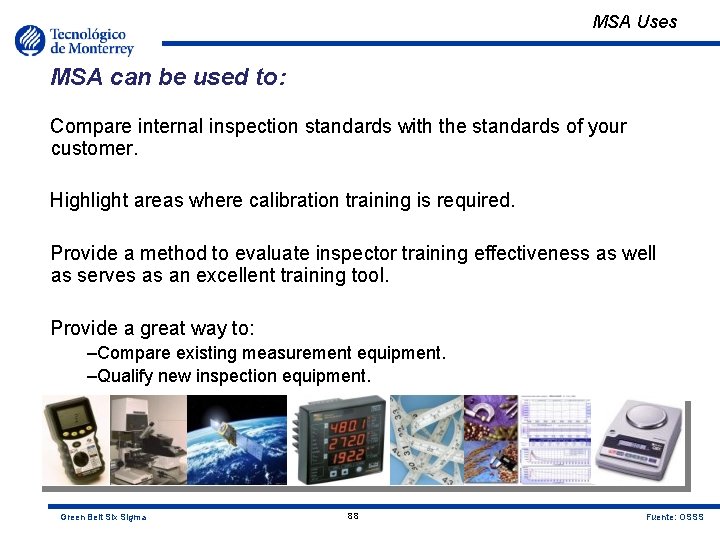
MSA Uses MSA can be used to: Compare internal inspection standards with the standards of your customer. Highlight areas where calibration training is required. Provide a method to evaluate inspector training effectiveness as well as serves as an excellent training tool. Provide a great way to: –Compare existing measurement equipment. –Qualify new inspection equipment. Green Belt Six Sigma 88 Fuente: OSSS

Why MSA? Measurement System Analysis is important to: • Study the % of variation in our process that is caused by our measurement system. • Compare measurements between operators. • Compare measurements between two (or more) measurement devices. • Provide criteria to accept new measurement systems (consider new equipment). • Evaluate a suspect gage. • Evaluate a gage before and after repair. • Determine true process variation. • Evaluate effectiveness of training program. Green Belt Six Sigma 89 Fuente: OSSS

Appropriate Measures are: • Sufficient – available to be measured regularly • Relevant –help to understand/isolate the problems • Representative - of the process across shifts and people • Contextual – collected with other relevant information that might explain process variability. Wadda ya wanna measure!? ! Green Belt Six Sigma 90 Fuente: OSSS

Poor Measures can result from: • Poor or non-existent operational definitions • Difficult measures • Poor sampling • Lack of understanding of the definitions • Inaccurate, insufficient or non-calibrated measurement devices Measurement Error compromises decisions that affect: • Customers • Producers • Suppliers Green Belt Six Sigma 91 Fuente: OSSS

Examples of What to Measure Examples of what and when to measure: • Primary and secondary metrics • Decision points in Process Maps • Any and all gauges, measurement devices, instruments, etc • “X’s” in the process • Prior to Hypothesis Testing • Prior to modeling • Prior to planning designed experiments • Before and after process changes • To qualify operators MSA is a Show Stopper!!! Green Belt Six Sigma 92 Fuente: OSSS

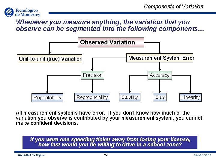
Components of Variation Whenever you measure anything, the variation that you observe can be segmented into the following components… Observed Variation Measurement System Error Unit-to-unit (true) Variation Precision Repeatability Accuracy Reproducibility Stability Bias Linearity All measurement systems have error. If you don’t know how much of the variation you observe is contributed by your measurement system, you cannot make confident decisions. If you were one speeding ticket away from losing your license, how fast would you be willing to drive in a school zone? Green Belt Six Sigma 93 Fuente: OSSS

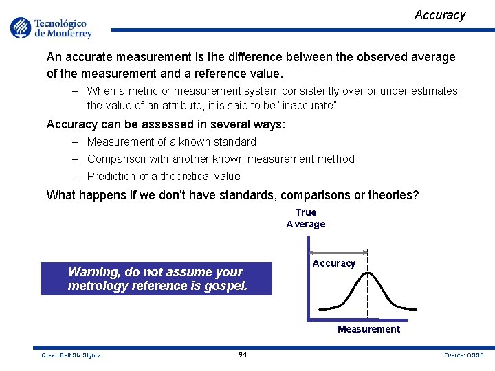
Accuracy An accurate measurement is the difference between the observed average of the measurement and a reference value. – When a metric or measurement system consistently over or under estimates the value of an attribute, it is said to be “inaccurate” Accuracy can be assessed in several ways: – Measurement of a known standard – Comparison with another known measurement method – Prediction of a theoretical value What happens if we don’t have standards, comparisons or theories? True Average Warning, do not assume your metrology reference is gospel. Accuracy Measurement Green Belt Six Sigma 94 Fuente: OSSS

Accuracy Against a Known Standard In transactional processes, the measurement system can consist of a database query. – For example, you may be interested in measuring product returns where you will want to analyze the details of the returns over some time period. – The query will provide you all the transaction details. However, before you invest a lot of time analyzing the data, you must ensure the data has integrity. – The analysis should include a comparison with known reference points. – For the example of product returns, the transaction details should add up to the same number that appears on financial reports, such as the income statement. Green Belt Six Sigma 95 Fuente: OSSS

Accuracy vs. Precision ACCURATE BOTH PRECISE = + Accuracy relates to how close the average of the shots are to the Master or bull's-eye. Precision relates to the spread of the shots or Variance. NEITHER Green Belt Six Sigma 96 Fuente: OSSS

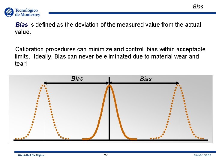
Bias is defined as the deviation of the measured value from the actual value. Calibration procedures can minimize and control bias within acceptable limits. Ideally, Bias can never be eliminated due to material wear and tear! Bias Green Belt Six Sigma Bias 97 Fuente: OSSS

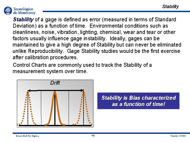
Stability of a gage is defined as error (measured in terms of Standard Deviation) as a function of time. Environmental conditions such as cleanliness, noise, vibration, lighting, chemical, wear and tear or other factors usually influence gage instability. Ideally, gages can be maintained to give a high degree of Stability but can never be eliminated unlike Reproducibility. Gage Stability studies would be the first exercise after calibration procedures. Control Charts are commonly used to track the Stability of a measurement system over time. Drift Stability is Bias characterized as a function of time! Green Belt Six Sigma 98 Fuente: OSSS

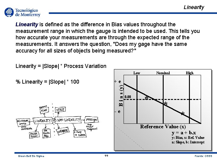
Linearity is defined as the difference in Bias values throughout the measurement range in which the gauge is intended to be used. This tells you how accurate your measurements are through the expected range of the measurements. It answers the question, "Does my gage have the same accuracy for all sizes of objects being measured? " Linearity = |Slope| * Process Variation Low Nominal High +e B i a s (y) % Linearity = |Slope| * 100 -e 0. 00 * * * Reference Value (x) y = a + b. x y: Bias, x: Ref. Value a: Slope, b: Intercept Green Belt Six Sigma 99 Fuente: OSSS

Precision A precise metric is one that returns the same value of a given attribute every time an estimate is made. Precise data are independent of who estimates them or when the estimate is made. Precision can be partitioned into two components: – Repeatability – Reproducibility Repeatability and Reproducibility = Gage R+R Green Belt Six Sigma 100 Fuente: OSSS

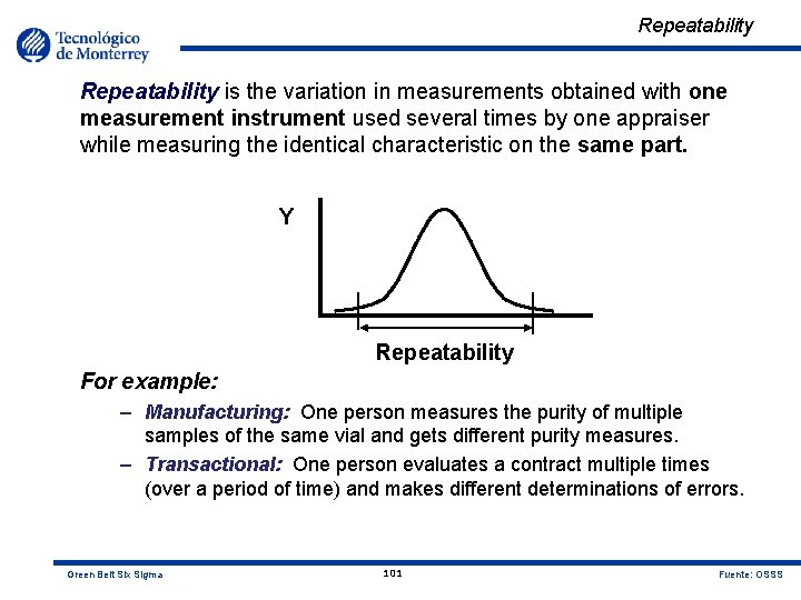
Repeatability is the variation in measurements obtained with one measurement instrument used several times by one appraiser while measuring the identical characteristic on the same part. Y Repeatability For example: – Manufacturing: One person measures the purity of multiple samples of the same vial and gets different purity measures. – Transactional: One person evaluates a contract multiple times (over a period of time) and makes different determinations of errors. Green Belt Six Sigma 101 Fuente: OSSS

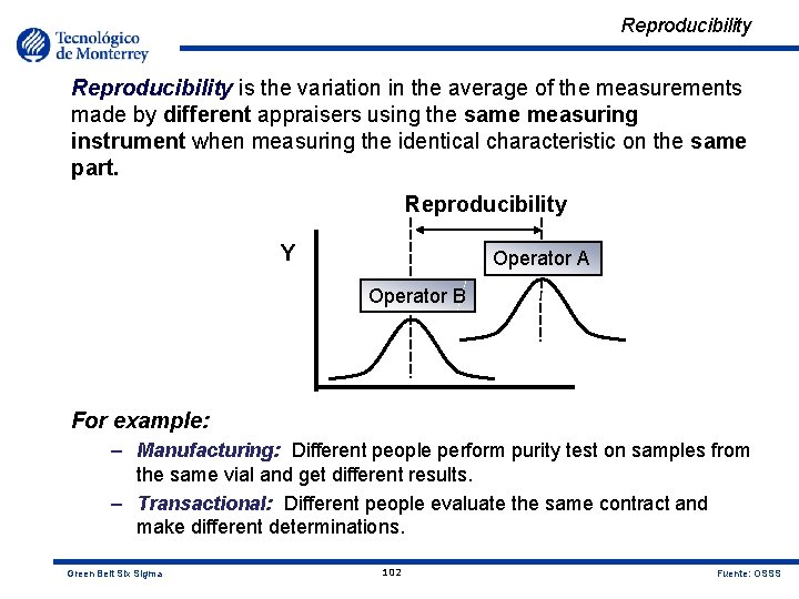
Reproducibility is the variation in the average of the measurements made by different appraisers using the same measuring instrument when measuring the identical characteristic on the same part. Reproducibility Y Operator A Operator B For example: – Manufacturing: Different people perform purity test on samples from the same vial and get different results. – Transactional: Different people evaluate the same contract and make different determinations. Green Belt Six Sigma 102 Fuente: OSSS

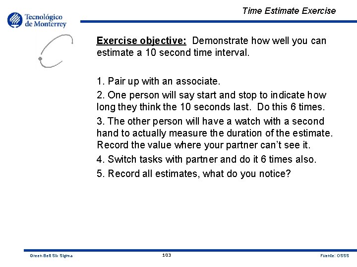
Time Estimate Exercise objective: Demonstrate how well you can estimate a 10 second time interval. 1. Pair up with an associate. 2. One person will say start and stop to indicate how long they think the 10 seconds last. Do this 6 times. 3. The other person will have a watch with a second hand to actually measure the duration of the estimate. Record the value where your partner can’t see it. 4. Switch tasks with partner and do it 6 times also. 5. Record all estimates, what do you notice? Green Belt Six Sigma 103 Fuente: OSSS

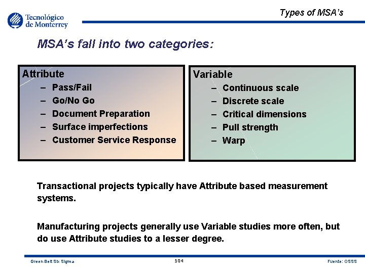
Types of MSA’s fall into two categories: Attribute Variable – – – – – Pass/Fail Go/No Go Document Preparation Surface imperfections Customer Service Response Continuous scale Discrete scale Critical dimensions Pull strength Warp Transactional projects typically have Attribute based measurement systems. Manufacturing projects generally use Variable studies more often, but do use Attribute studies to a lesser degree. Green Belt Six Sigma 104 Fuente: OSSS

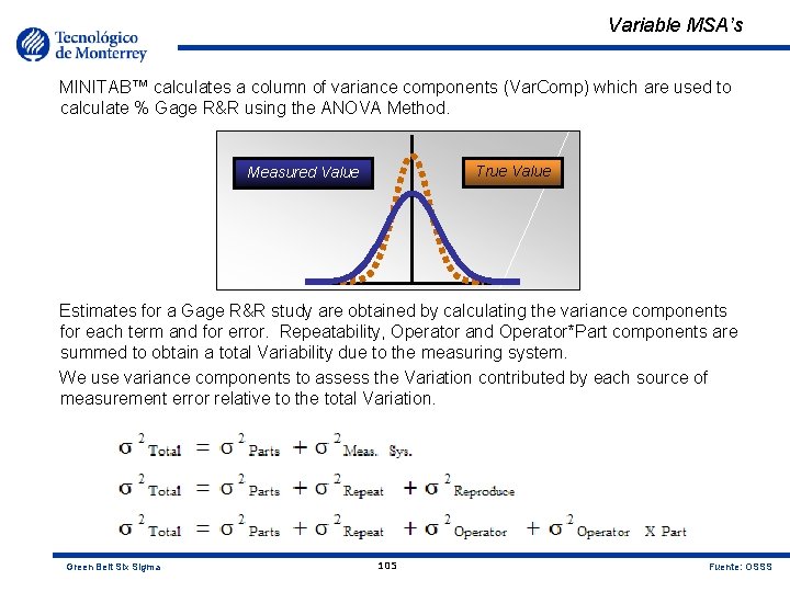
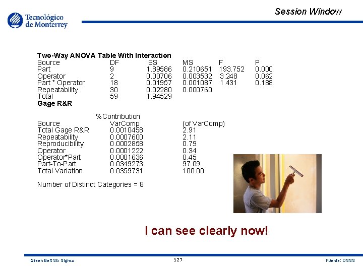
Variable MSA’s MINITAB™ calculates a column of variance components (Var. Comp) which are used to calculate % Gage R&R using the ANOVA Method. True Value Measured Value Estimates for a Gage R&R study are obtained by calculating the variance components for each term and for error. Repeatability, Operator and Operator*Part components are summed to obtain a total Variability due to the measuring system. We use variance components to assess the Variation contributed by each source of measurement error relative to the total Variation. Green Belt Six Sigma 105 Fuente: OSSS

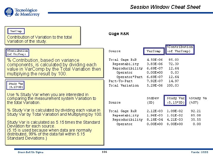
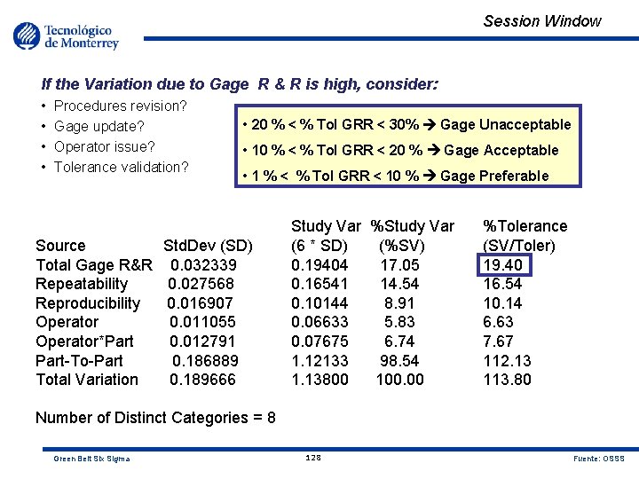
Session Window Cheat Sheet Contribution of Variation to the total Variation of the study. % Contribution, based on variance components, is calculated by dividing each value in Var. Comp by the Total Variation then multiplying the result by 100. Use % Study Var when you are interested in comparing the measurement system Variation to the total Variation. % Study Var is calculated by dividing each value in Study Var by Total Variation and Multiplying by 100. Study Var is calculated as 5. 15 times the Standard Deviation for each source. (5. 15 is used because when data are normally distributed, 99% of the data fall within 5. 15 Standard Deviations. ) Green Belt Six Sigma 106 Fuente: OSSS

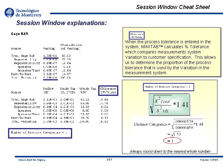
Session Window Cheat Sheet Session Window explanations: When the process tolerance is entered in the system, MINITABTM calculates % Tolerance which compares measurements system Variation to customer specification. This allows us to determine the proportion of the process tolerance that is used by the Variation in the measurement system. Always round down to the nearest whole number. Green Belt Six Sigma 107 Fuente: OSSS

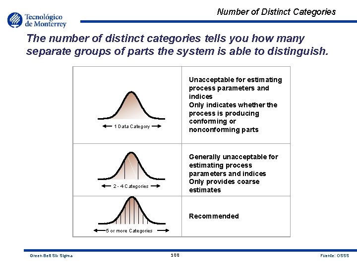
Number of Distinct Categories The number of distinct categories tells you how many separate groups of parts the system is able to distinguish. Unacceptable for estimating process parameters and indices Only indicates whether the process is producing conforming or nonconforming parts 1 Data Category Generally unacceptable for estimating process parameters and indices Only provides coarse estimates 2 - 4 Categories Recommended 5 or more Categories Green Belt Six Sigma 108 Fuente: OSSS

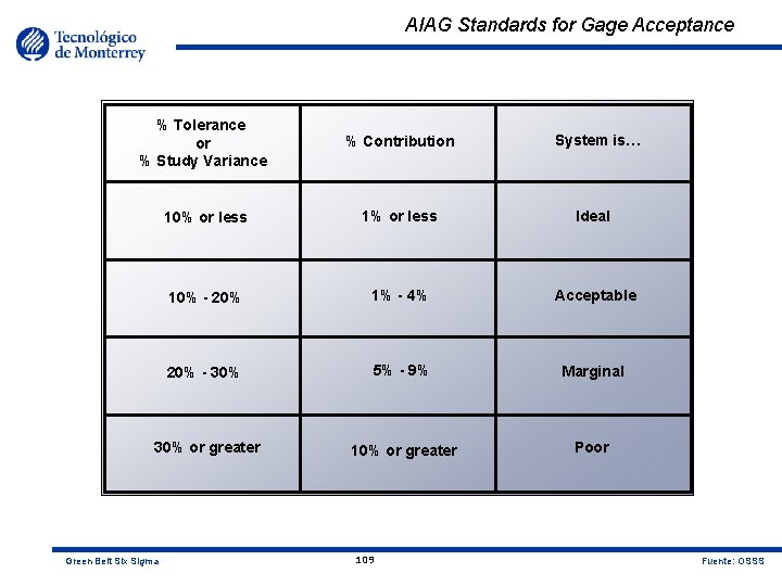
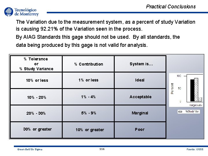
AIAG Standards for Gage Acceptance % Tolerance or % Study Variance % Contribution 10% or less 1% or less Ideal 10% - 20% 1% - 4% Acceptable 20% - 30% 5% - 9% Marginal 30% or greater 10% or greater Poor Green Belt Six Sigma 109 System is… Fuente: OSSS

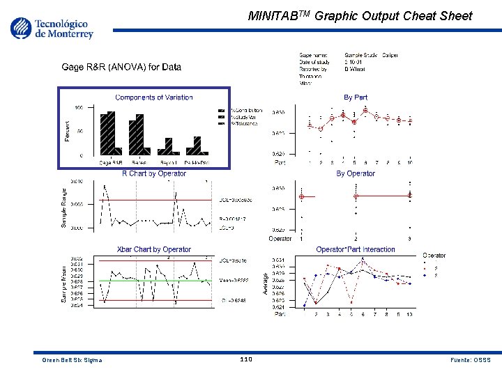
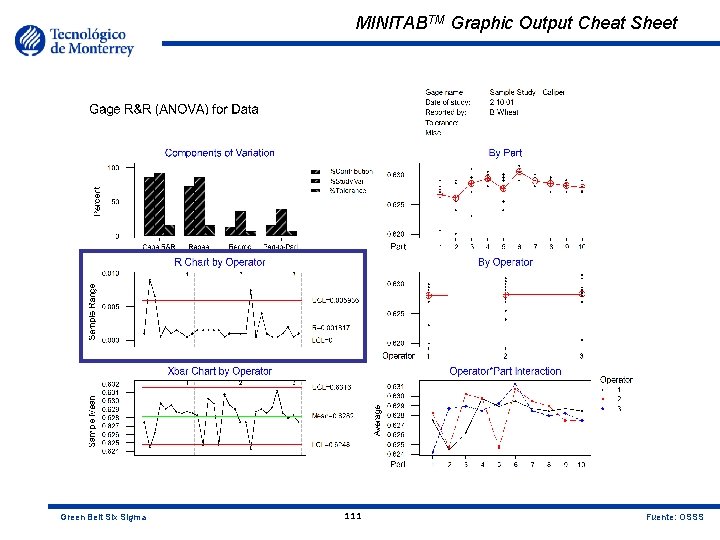
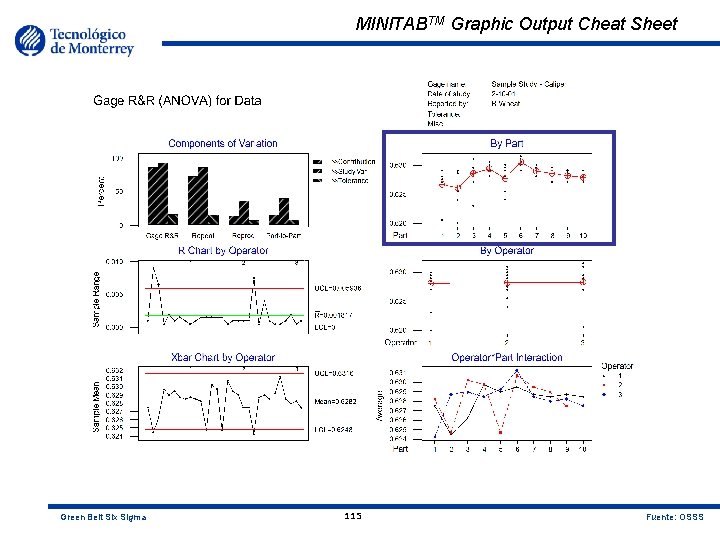
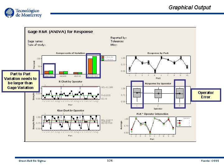
MINITABTM Graphic Output Cheat Sheet Green Belt Six Sigma 110 Fuente: OSSS

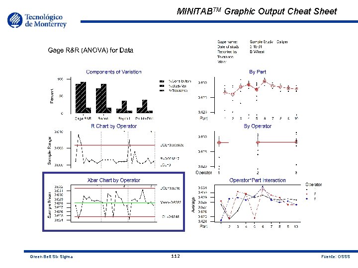
MINITABTM Graphic Output Cheat Sheet Green Belt Six Sigma 111 Fuente: OSSS

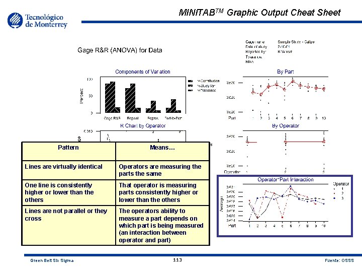
MINITABTM Graphic Output Cheat Sheet Green Belt Six Sigma 112 Fuente: OSSS

MINITABTM Graphic Output Cheat Sheet Pattern Means… Lines are virtually identical Operators are measuring the parts the same One line is consistently higher or lower than the others That operator is measuring parts consistently higher or lower than the others Lines are not parallel or they cross The operators ability to measure a part depends on which part is being measured (an interaction between operator and part) Green Belt Six Sigma 113 Fuente: OSSS

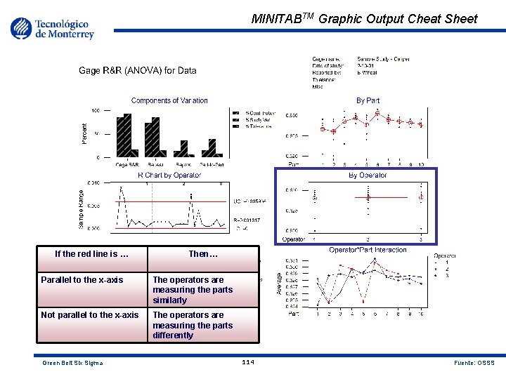
MINITABTM Graphic Output Cheat Sheet If the red line is … Then… Parallel to the x-axis The operators are measuring the parts similarly Not parallel to the x-axis The operators are measuring the parts differently Green Belt Six Sigma 114 Fuente: OSSS

MINITABTM Graphic Output Cheat Sheet Green Belt Six Sigma 115 Fuente: OSSS

Practical Conclusions The Variation due to the measurement system, as a percent of study Variation is causing 92. 21% of the Variation seen in the process. By AIAG Standards this gage should not be used. By all standards, the data being produced by this gage is not valid for analysis. % Tolerance or % Study Variance % Contribution 10% or less 1% or less Ideal 10% - 20% 1% - 4% Acceptable 20% - 30% 5% - 9% Marginal 30% or greater 10% or greater Poor Green Belt Six Sigma 116 System is… Fuente: OSSS

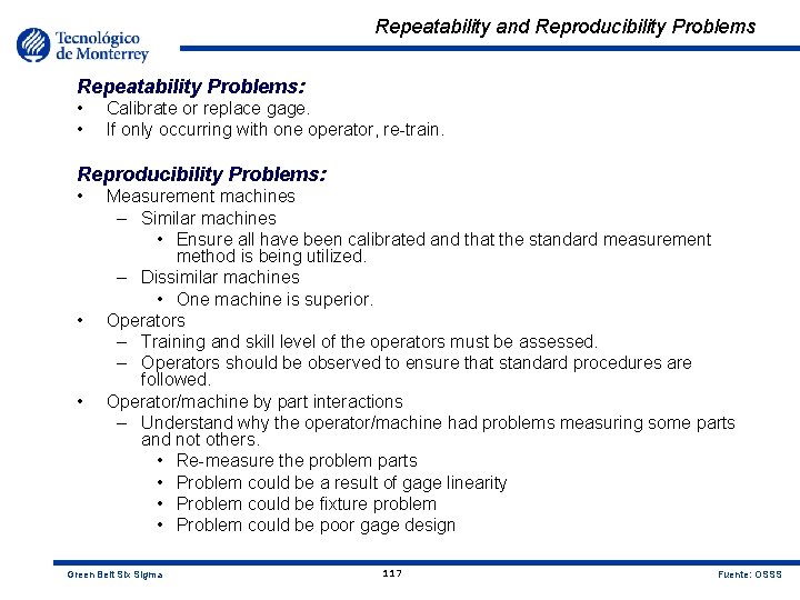
Repeatability and Reproducibility Problems Repeatability Problems: • • Calibrate or replace gage. If only occurring with one operator, re-train. Reproducibility Problems: • • • Measurement machines – Similar machines • Ensure all have been calibrated and that the standard measurement method is being utilized. – Dissimilar machines • One machine is superior. Operators – Training and skill level of the operators must be assessed. – Operators should be observed to ensure that standard procedures are followed. Operator/machine by part interactions – Understand why the operator/machine had problems measuring some parts and not others. • Re-measure the problem parts • Problem could be a result of gage linearity • Problem could be fixture problem • Problem could be poor gage design Green Belt Six Sigma 117 Fuente: OSSS

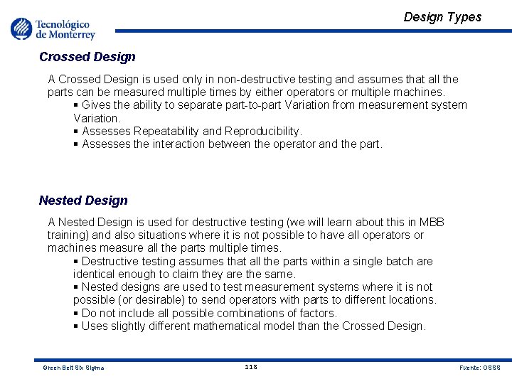
Design Types Crossed Design A Crossed Design is used only in non-destructive testing and assumes that all the parts can be measured multiple times by either operators or multiple machines. § Gives the ability to separate part-to-part Variation from measurement system Variation. § Assesses Repeatability and Reproducibility. § Assesses the interaction between the operator and the part. Nested Design A Nested Design is used for destructive testing (we will learn about this in MBB training) and also situations where it is not possible to have all operators or machines measure all the parts multiple times. § Destructive testing assumes that all the parts within a single batch are identical enough to claim they are the same. § Nested designs are used to test measurement systems where it is not possible (or desirable) to send operators with parts to different locations. § Do not include all possible combinations of factors. § Uses slightly different mathematical model than the Crossed Design. Green Belt Six Sigma 118 Fuente: OSSS

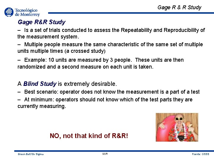
Gage R & R Study Gage R&R Study – Is a set of trials conducted to assess the Repeatability and Reproducibility of the measurement system. – Multiple people measure the same characteristic of the same set of multiple units multiple times (a crossed study) – Example: 10 units are measured by 3 people. These units are then randomized and a second measure on each unit is taken. A Blind Study is extremely desirable. – Best scenario: operator does not know the measurement is a part of a test – At minimum: operators should not know which of the test parts they are currently measuring. NO, not that kind of R&R! Green Belt Six Sigma 119 Fuente: OSSS

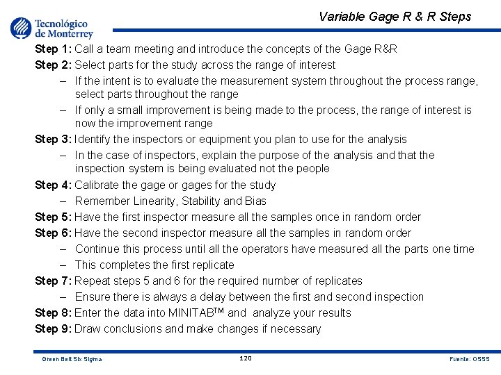
Variable Gage R & R Steps Step 1: Call a team meeting and introduce the concepts of the Gage R&R Step 2: Select parts for the study across the range of interest – If the intent is to evaluate the measurement system throughout the process range, select parts throughout the range – If only a small improvement is being made to the process, the range of interest is now the improvement range Step 3: Identify the inspectors or equipment you plan to use for the analysis – In the case of inspectors, explain the purpose of the analysis and that the inspection system is being evaluated not the people Step 4: Calibrate the gage or gages for the study – Remember Linearity, Stability and Bias Step 5: Have the first inspector measure all the samples once in random order Step 6: Have the second inspector measure all the samples in random order – Continue this process until all the operators have measured all the parts one time – This completes the first replicate Step 7: Repeat steps 5 and 6 for the required number of replicates – Ensure there is always a delay between the first and second inspection Step 8: Enter the data into MINITABTM and analyze your results Step 9: Draw conclusions and make changes if necessary Green Belt Six Sigma 120 Fuente: OSSS

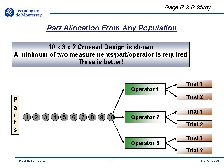
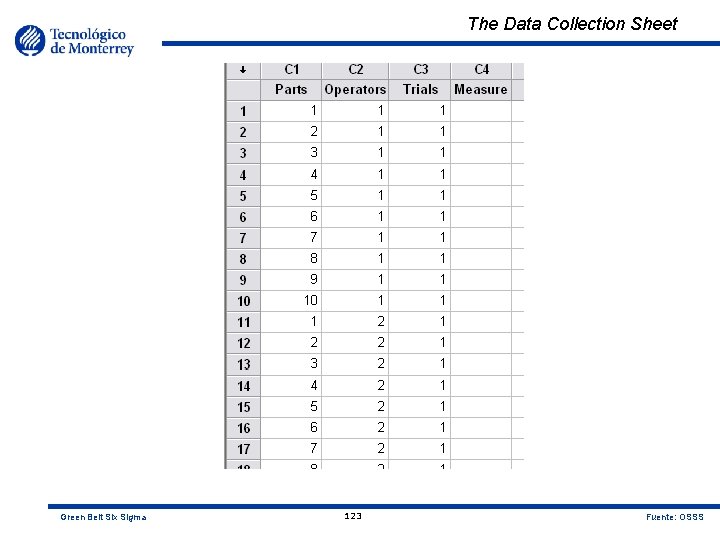
Gage R & R Study Part Allocation From Any Population 10 x 3 x 2 Crossed Design is shown A minimum of two measurements/part/operator is required Three is better! Operator 1 P a r t s Trial 1 Trial 2 1 2 3 4 5 6 7 8 9 10 Operator 2 Trial 1 Trial 2 Operator 3 Trial 1 Trial 2 Green Belt Six Sigma 121 Fuente: OSSS

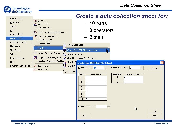
Data Collection Sheet Create a data collection sheet for: – 10 parts – 3 operators – 2 trials Green Belt Six Sigma 122 Fuente: OSSS

The Data Collection Sheet Green Belt Six Sigma 123 Fuente: OSSS

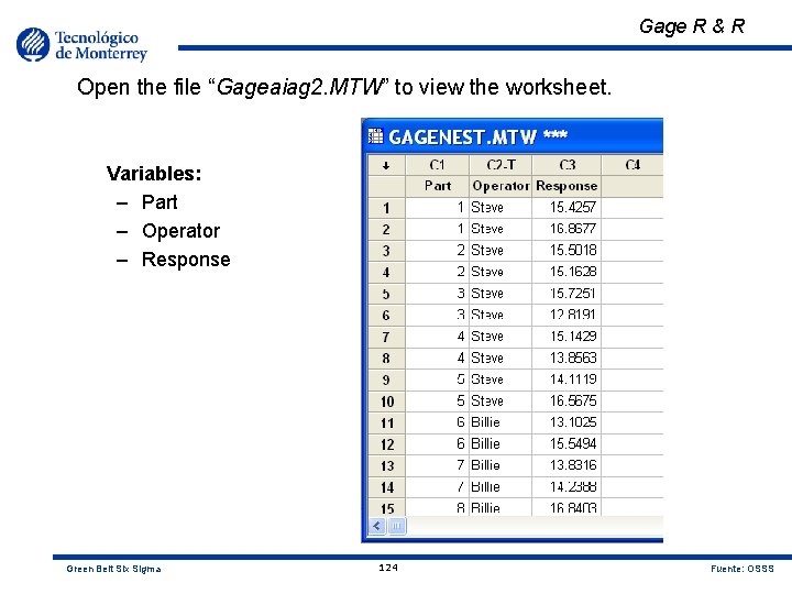
Gage R & R Open the file “Gageaiag 2. MTW” to view the worksheet. Variables: – Part – Operator – Response Green Belt Six Sigma 124 Fuente: OSSS

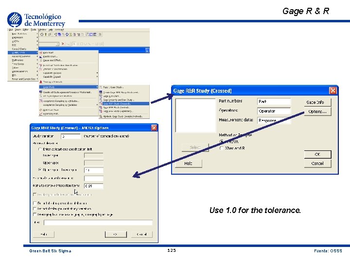
Gage R & R Use 1. 0 for the tolerance. Green Belt Six Sigma 125 Fuente: OSSS

Graphical Output Part to Part Variation needs to be larger than Gage Variation Operator Error Green Belt Six Sigma 126 Fuente: OSSS

Session Window Two-Way ANOVA Table With Interaction Source DF SS Part 9 1. 89586 Operator 2 0. 00706 Part * Operator 18 0. 01957 Repeatability 30 0. 02280 Total 59 1. 94529 Gage R&R Source Total Gage R&R Repeatability Reproducibility Operator*Part-To-Part Total Variation MS F 0. 210651 193. 752 0. 003532 3. 248 0. 001087 1. 431 0. 000760 %Contribution Var. Comp 0. 0010458 0. 0007600 0. 0002858 0. 0001222 0. 0001636 0. 0349273 0. 0359731 P 0. 000 0. 062 0. 188 (of Var. Comp) 2. 91 2. 11 0. 79 0. 34 0. 45 97. 09 100. 00 Number of Distinct Categories = 8 I can see clearly now! Green Belt Six Sigma 127 Fuente: OSSS

Session Window If the Variation due to Gage R & R is high, consider: • • Procedures revision? Gage update? Operator issue? Tolerance validation? • 20 % < % Tol GRR < 30% Gage Unacceptable • 10 % < % Tol GRR < 20 % Gage Acceptable • 1 % < % Tol GRR < 10 % Gage Preferable Source Std. Dev (SD) Total Gage R&R 0. 032339 Repeatability 0. 027568 Reproducibility 0. 016907 Operator 0. 011055 Operator*Part 0. 012791 Part-To-Part 0. 186889 Total Variation 0. 189666 Study Var %Study Var (6 * SD) (%SV) 0. 19404 17. 05 0. 16541 14. 54 0. 10144 8. 91 0. 06633 5. 83 0. 07675 6. 74 1. 12133 98. 54 1. 13800 100. 00 %Tolerance (SV/Toler) 19. 40 16. 54 10. 14 6. 63 7. 67 112. 13 113. 80 Number of Distinct Categories = 8 Green Belt Six Sigma 128 Fuente: OSSS

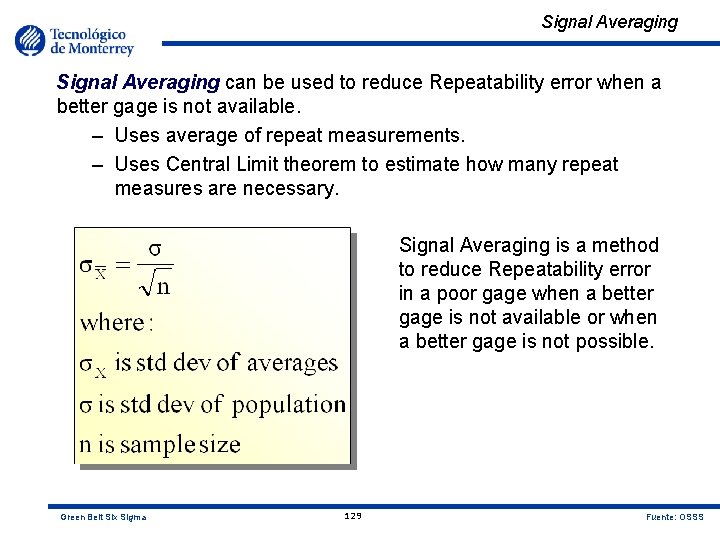
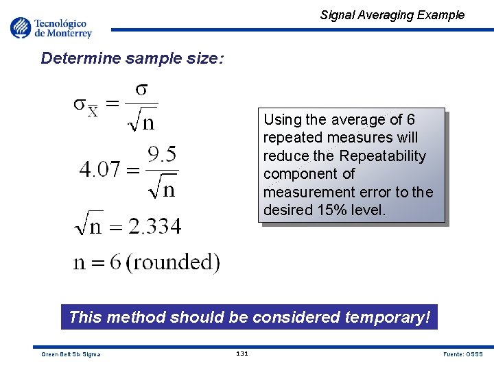
Signal Averaging can be used to reduce Repeatability error when a better gage is not available. – Uses average of repeat measurements. – Uses Central Limit theorem to estimate how many repeat measures are necessary. Signal Averaging is a method to reduce Repeatability error in a poor gage when a better gage is not available or when a better gage is not possible. Green Belt Six Sigma 129 Fuente: OSSS

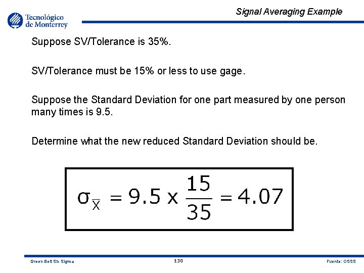
Signal Averaging Example Suppose SV/Tolerance is 35%. SV/Tolerance must be 15% or less to use gage. Suppose the Standard Deviation for one part measured by one person many times is 9. 5. Determine what the new reduced Standard Deviation should be. Green Belt Six Sigma 130 Fuente: OSSS

Signal Averaging Example Determine sample size: Using the average of 6 repeated measures will reduce the Repeatability component of measurement error to the desired 15% level. This method should be considered temporary! Green Belt Six Sigma 131 Fuente: OSSS

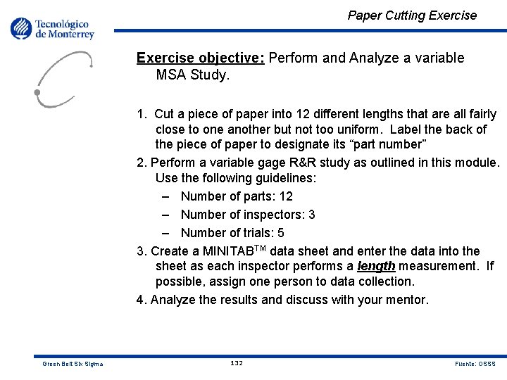
Paper Cutting Exercise objective: Perform and Analyze a variable MSA Study. 1. Cut a piece of paper into 12 different lengths that are all fairly close to one another but not too uniform. Label the back of the piece of paper to designate its “part number” 2. Perform a variable gage R&R study as outlined in this module. Use the following guidelines: – Number of parts: 12 – Number of inspectors: 3 – Number of trials: 5 3. Create a MINITABTM data sheet and enter the data into the sheet as each inspector performs a length measurement. If possible, assign one person to data collection. 4. Analyze the results and discuss with your mentor. Green Belt Six Sigma 132 Fuente: OSSS

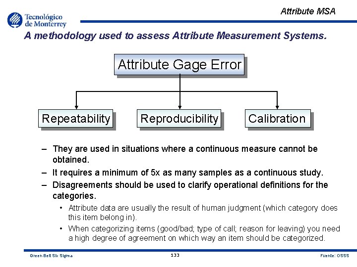
Attribute MSA A methodology used to assess Attribute Measurement Systems. Attribute Gage Error Repeatability Reproducibility Calibration – They are used in situations where a continuous measure cannot be obtained. – It requires a minimum of 5 x as many samples as a continuous study. – Disagreements should be used to clarify operational definitions for the categories. • Attribute data are usually the result of human judgment (which category does this item belong in). • When categorizing items (good/bad; type of call; reason for leaving) you need a high degree of agreement on which way an item should be categorized. Green Belt Six Sigma 133 Fuente: OSSS

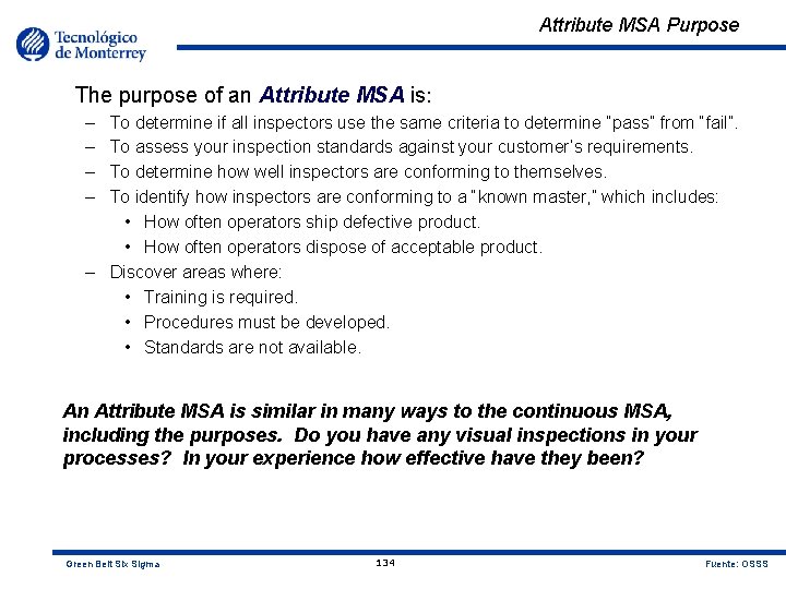
Attribute MSA Purpose The purpose of an Attribute MSA is: – – To determine if all inspectors use the same criteria to determine “pass” from “fail”. To assess your inspection standards against your customer’s requirements. To determine how well inspectors are conforming to themselves. To identify how inspectors are conforming to a “known master, ” which includes: • How often operators ship defective product. • How often operators dispose of acceptable product. – Discover areas where: • Training is required. • Procedures must be developed. • Standards are not available. An Attribute MSA is similar in many ways to the continuous MSA, including the purposes. Do you have any visual inspections in your processes? In your experience how effective have they been? Green Belt Six Sigma 134 Fuente: OSSS

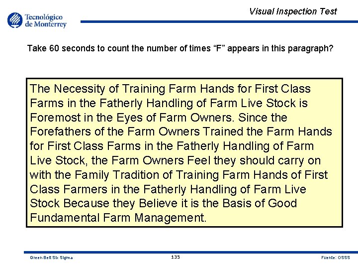
Visual Inspection Test Take 60 seconds to count the number of times “F” appears in this paragraph? The Necessity of Training Farm Hands for First Class Farms in the Fatherly Handling of Farm Live Stock is Foremost in the Eyes of Farm Owners. Since the Forefathers of the Farm Owners Trained the Farm Hands for First Class Farms in the Fatherly Handling of Farm Live Stock, the Farm Owners Feel they should carry on with the Family Tradition of Training Farm Hands of First Class Farmers in the Fatherly Handling of Farm Live Stock Because they Believe it is the Basis of Good Fundamental Farm Management. Green Belt Six Sigma 135 Fuente: OSSS

How can we Improve Visual Inspection? Visual Inspection can be improved by: • • • Operator Training & Certification Develop Visual Aids/Boundary Samples Establish Standards Establish Set-Up Procedures Establish Evaluation Procedures – Evaluation of the same location on each part. – Each evaluation performed under the same lighting. – Ensure all evaluations are made with the same standard. Look closely now! Green Belt Six Sigma 136 Fuente: OSSS

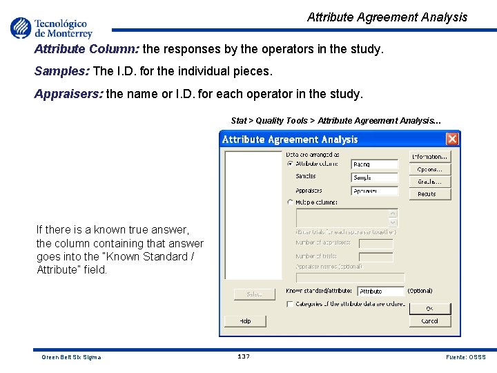
Attribute Agreement Analysis Attribute Column: the responses by the operators in the study. Samples: The I. D. for the individual pieces. Appraisers: the name or I. D. for each operator in the study. Stat > Quality Tools > Attribute Agreement Analysis… If there is a known true answer, the column containing that answer goes into the “Known Standard / Attribute” field. Green Belt Six Sigma 137 Fuente: OSSS

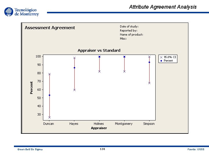
Attribute Agreement Analysis Green Belt Six Sigma 138 Fuente: OSSS

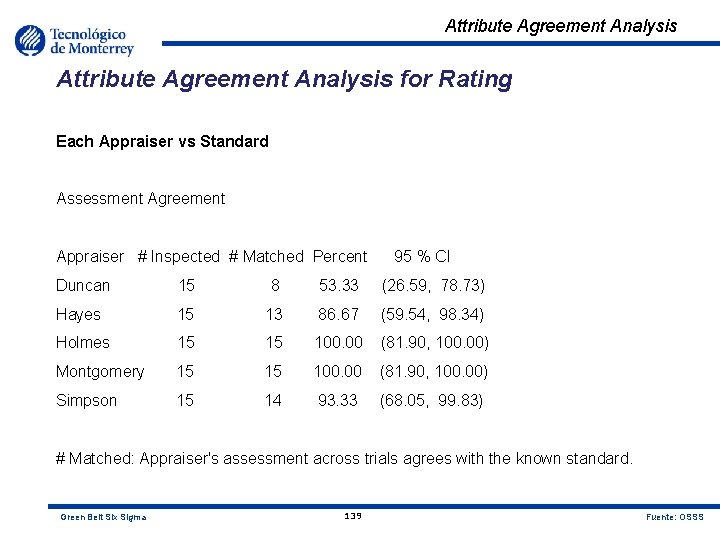
Attribute Agreement Analysis for Rating Each Appraiser vs Standard Assessment Agreement Appraiser # Inspected # Matched Percent 95 % CI Duncan 15 8 53. 33 (26. 59, 78. 73) Hayes 15 13 86. 67 (59. 54, 98. 34) Holmes 15 15 100. 00 (81. 90, 100. 00) Montgomery 15 15 100. 00 (81. 90, 100. 00) Simpson 15 14 93. 33 (68. 05, 99. 83) # Matched: Appraiser's assessment across trials agrees with the known standard. Green Belt Six Sigma 139 Fuente: OSSS

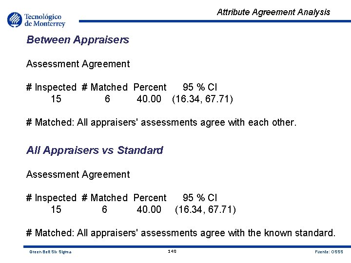
Attribute Agreement Analysis Between Appraisers Assessment Agreement # Inspected # Matched Percent 95 % CI 15 6 40. 00 (16. 34, 67. 71) # Matched: All appraisers' assessments agree with each other. All Appraisers vs Standard Assessment Agreement # Inspected # Matched Percent 95 % CI 15 6 40. 00 (16. 34, 67. 71) # Matched: All appraisers' assessments agree with the known standard. Green Belt Six Sigma 140 Fuente: OSSS

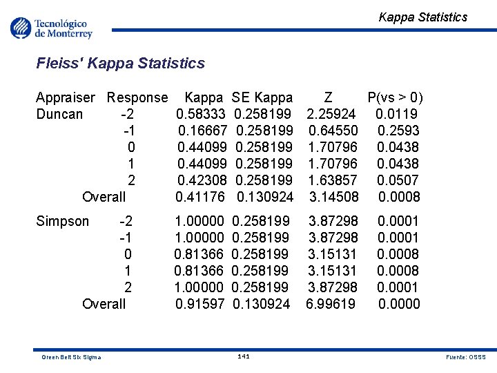
Kappa Statistics Fleiss' Kappa Statistics Appraiser Response Kappa SE Kappa Duncan -2 0. 58333 0. 258199 -1 0. 16667 0. 258199 0 0. 44099 0. 258199 1 0. 44099 0. 258199 2 0. 42308 0. 258199 Overall 0. 41176 0. 130924 Z P(vs > 0) 2. 25924 0. 0119 0. 64550 0. 2593 1. 70796 0. 0438 1. 63857 0. 0507 3. 14508 0. 0008 Simpson 3. 87298 3. 15131 3. 87298 6. 99619 -2 -1 0 1 2 Overall Green Belt Six Sigma 1. 00000 0. 81366 1. 00000 0. 91597 0. 258199 0. 130924 141 0. 0001 0. 0008 0. 0001 0. 0000 Fuente: OSSS

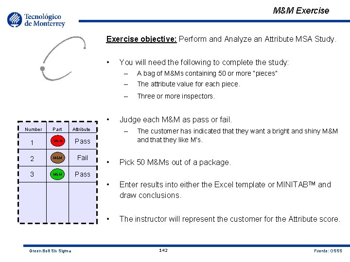
M&M Exercise objective: Perform and Analyze an Attribute MSA Study. • • Number Part Attribute 1 M&M Pass 2 M&M Fail 3 M&M Pass Green Belt Six Sigma You will need the following to complete the study: – A bag of M&Ms containing 50 or more “pieces” – The attribute value for each piece. – Three or more inspectors. Judge each M&M as pass or fail. – The customer has indicated that they want a bright and shiny M&M and that they like M’s. • Pick 50 M&Ms out of a package. • Enter results into either the Excel template or MINITABTM and draw conclusions. • The instructor will represent the customer for the Attribute score. 142 Fuente: OSSS

Summary At this point, you should be able to: • Understand Precision & Accuracy • Understand Bias, Linearity and Stability • Understand Repeatability & Reproducibility • Understand the impact of poor gage capability on product quality • Identify the various components of Variation • Perform the step by step methodology in Variable and Attribute MSA’s Green Belt Six Sigma 143 Fuente: OSSS

Measure Phase Process Capability

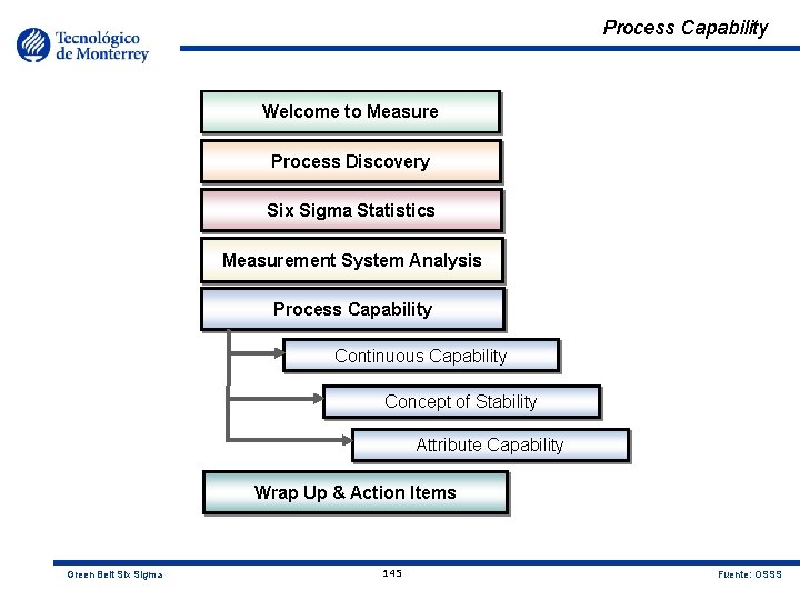
Process Capability Welcome to Measure Process Discovery Six Sigma Statistics Measurement System Analysis Process Capability Continuous Capability Concept of Stability Attribute Capability Wrap Up & Action Items Green Belt Six Sigma 145 Fuente: OSSS

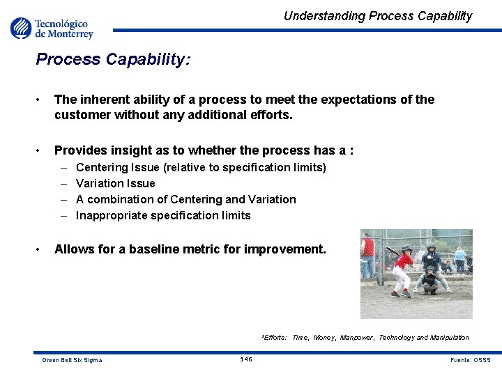
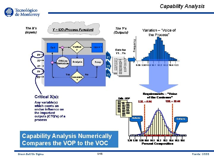
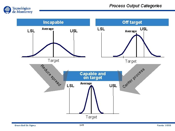
Understanding Process Capability: • The inherent ability of a process to meet the expectations of the customer without any additional efforts. • Provides insight as to whether the process has a : – – • Centering Issue (relative to specification limits) Variation Issue A combination of Centering and Variation Inappropriate specification limits Allows for a baseline metric for improvement. *Efforts: Time, Money, Manpower, Technology and Manipulation Green Belt Six Sigma 146 Fuente: OSSS

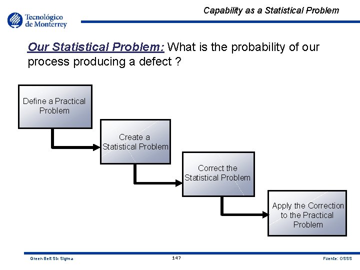
Capability as a Statistical Problem Our Statistical Problem: What is the probability of our process producing a defect ? Define a Practical Problem Create a Statistical Problem Correct the Statistical Problem Apply the Correction to the Practical Problem Green Belt Six Sigma 147 Fuente: OSSS

Capability Analysis Numerically Compares the VOP to the VOC Green Belt Six Sigma 148 Fuente: OSSS

Process Output Categories Incapable LSL Average Off target LSL USL Average Target d Re e uc Capable and on target re sp ad LSL Average USL r rp ss e c o e t en C Target Green Belt Six Sigma 149 Fuente: OSSS

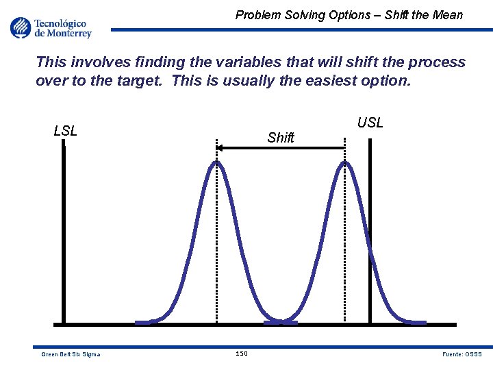
Problem Solving Options – Shift the Mean This involves finding the variables that will shift the process over to the target. This is usually the easiest option. USL LSL Green Belt Six Sigma Shift 150 Fuente: OSSS

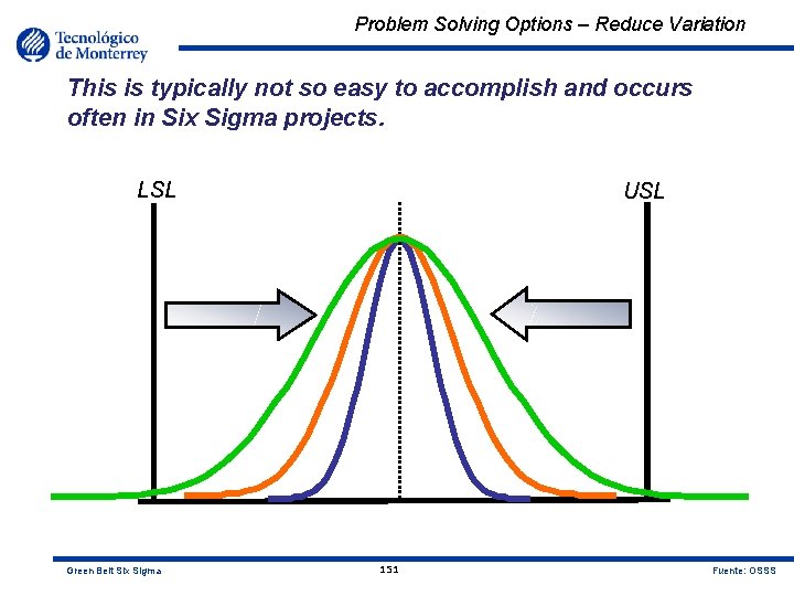
Problem Solving Options – Reduce Variation This is typically not so easy to accomplish and occurs often in Six Sigma projects. LSL Green Belt Six Sigma USL 151 Fuente: OSSS

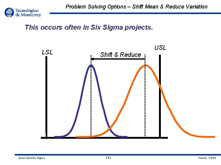
Problem Solving Options – Shift Mean & Reduce Variation This occurs often in Six Sigma projects. LSL Green Belt Six Sigma USL Shift & Reduce 152 Fuente: OSSS

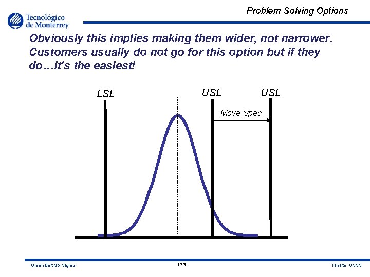
Problem Solving Options Obviously this implies making them wider, not narrower. Customers usually do not go for this option but if they do…it’s the easiest! USL LSL USL Move Spec Green Belt Six Sigma 153 Fuente: OSSS

Capability Studies: • Are intended to be regular, periodic, estimations of a process’s ability to meet its requirements. • Can be conducted on both Discrete and Continuous Data. • Are most meaningful when conducted on stable, predictable processes. • Are commonly reported as Sigma Level which is optimal (short term) performance. • Require a thorough understanding of the following: – – – Customer’s or business’s specification limits Nature of long-term vs. short-term data Mean and Standard Deviation of the process Assessment of the Normality of the data (Continuous Data only) Procedure for determining Sigma level Green Belt Six Sigma 154 Fuente: OSSS

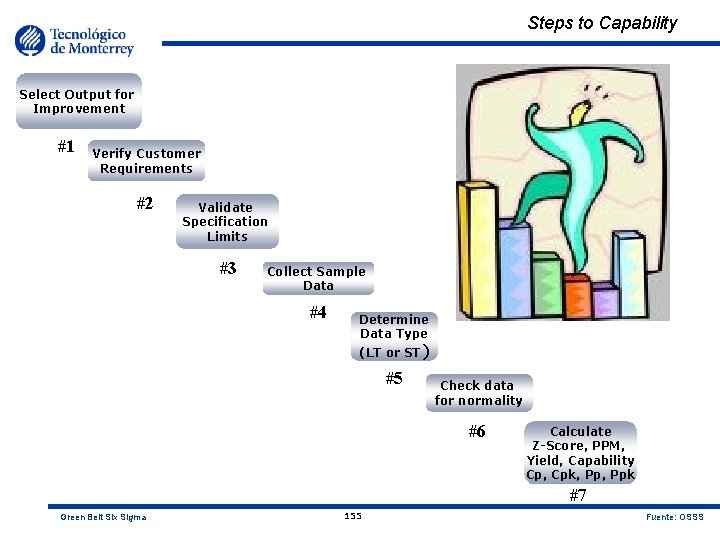
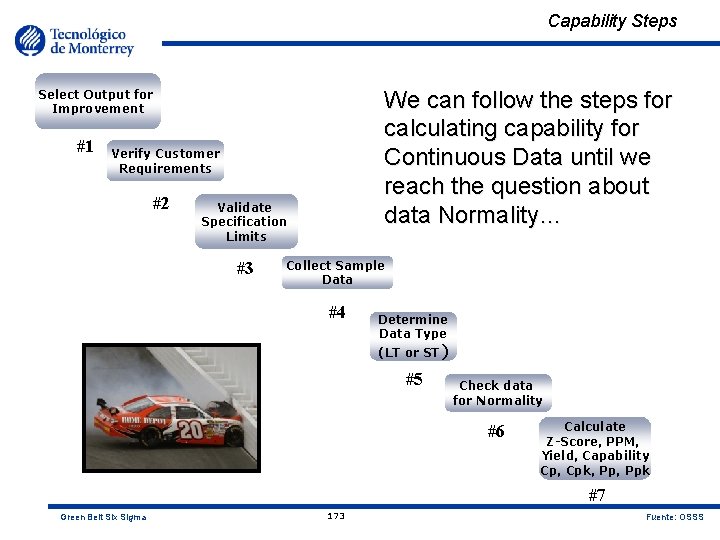
Steps to Capability Select Output for Improvement #1 Verify Customer Requirements #2 Validate Specification Limits #3 Collect Sample Data #4 Determine Data Type (LT or ST) #5 Check data for normality #6 Calculate Z-Score, PPM, Yield, Capability Cp, Cpk, Ppk #7 Green Belt Six Sigma 155 Fuente: OSSS

Verifying the Specifications Questions to consider: • What is the source of the specifications? – – Customer requirements (VOC) Business requirements (target, benchmark) Compliance requirements (regulations) Design requirements (blueprint, system) • Are they current? Likely to change? • Are they understood and agreed upon? – Operational definitions – Deployed to the work force Green Belt Six Sigma 156 Fuente: OSSS

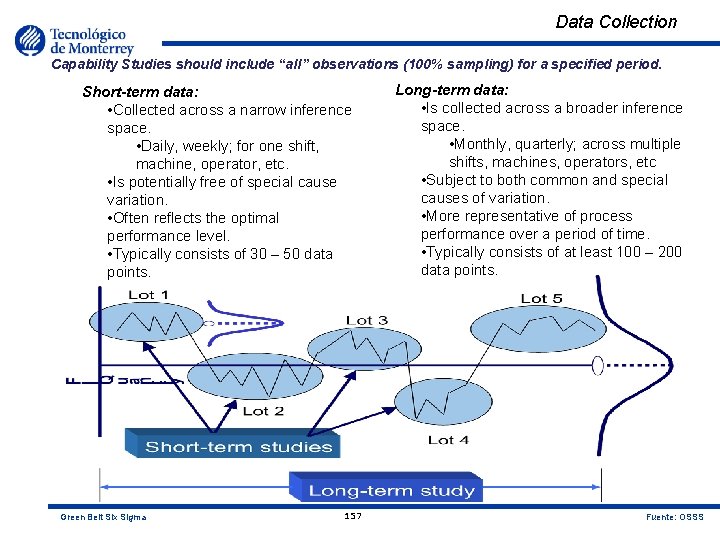
Data Collection Capability Studies should include “all” observations (100% sampling) for a specified period. Short-term data: • Collected across a narrow inference space. • Daily, weekly; for one shift, machine, operator, etc. • Is potentially free of special cause variation. • Often reflects the optimal performance level. • Typically consists of 30 – 50 data points. Green Belt Six Sigma 157 Long-term data: • Is collected across a broader inference space. • Monthly, quarterly; across multiple shifts, machines, operators, etc • Subject to both common and special causes of variation. • More representative of process performance over a period of time. • Typically consists of at least 100 – 200 data points. Fuente: OSSS

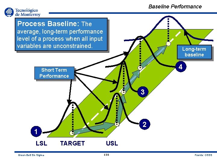
Baseline Performance Process Baseline: The average, long-term performance level of a process when all input variables are unconstrained. Long-term baseline 4 Short Term Performance ` 2 1 LSL Green Belt Six Sigma 3 TARGET USL 158 Fuente: OSSS

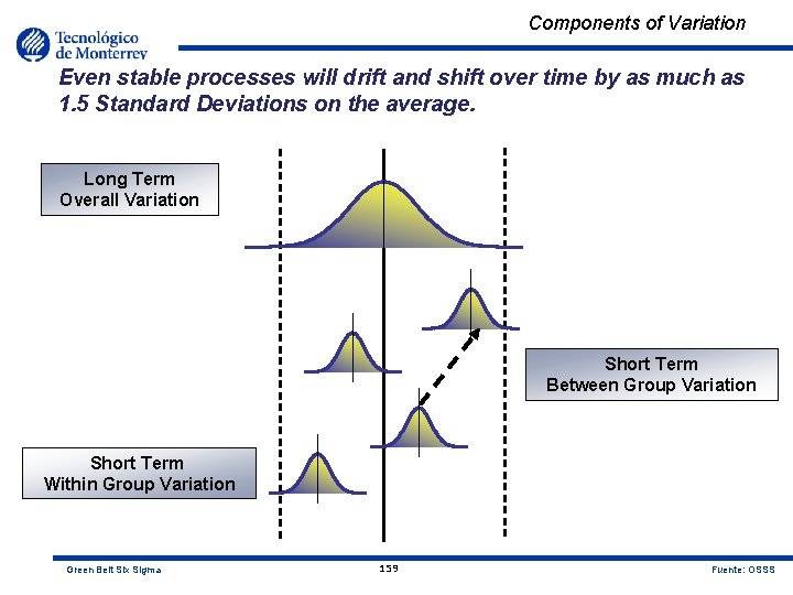
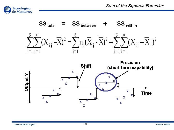
Components of Variation Even stable processes will drift and shift over time by as much as 1. 5 Standard Deviations on the average. Long Term Overall Variation Short Term Between Group Variation Short Term Within Group Variation Green Belt Six Sigma 159 Fuente: OSSS

Sum of the Squares Formulas = SS total + SS between Precision (short-term capability) Shift Output Y x x Green Belt Six Sigma x x x SS within x x x x x 160 x x x x Time x Fuente: OSSS

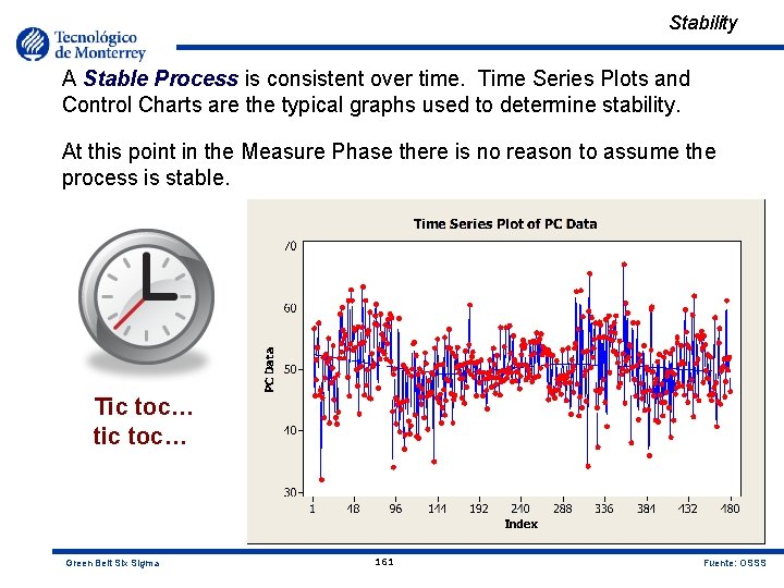
Stability A Stable Process is consistent over time. Time Series Plots and Control Charts are the typical graphs used to determine stability. At this point in the Measure Phase there is no reason to assume the process is stable. Tic toc… tic toc… Green Belt Six Sigma 161 Fuente: OSSS

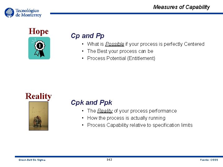
Measures of Capability Hope Cp and Pp • What is Possible if your process is perfectly Centered • The Best your process can be • Process Potential (Entitlement) Reality Cpk and Ppk • The Reality of your process performance • How the process is actually running • Process Capability relative to specification limits Green Belt Six Sigma 162 Fuente: OSSS

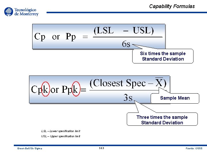
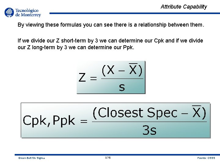
Capability Formulas Six times the sample Standard Deviation Sample Mean Three times the sample Standard Deviation LSL – Lower specification limit USL – Upper specification limit Green Belt Six Sigma 163 Fuente: OSSS

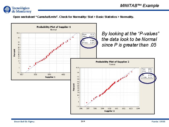
MINITAB™ Example Open worksheet “Camshaft. mtw”. Check for Normality: Stat > Basic Statistics > Normality. By looking at the “P-values” the data look to be Normal since P is greater than. 05 Green Belt Six Sigma 164 Fuente: OSSS

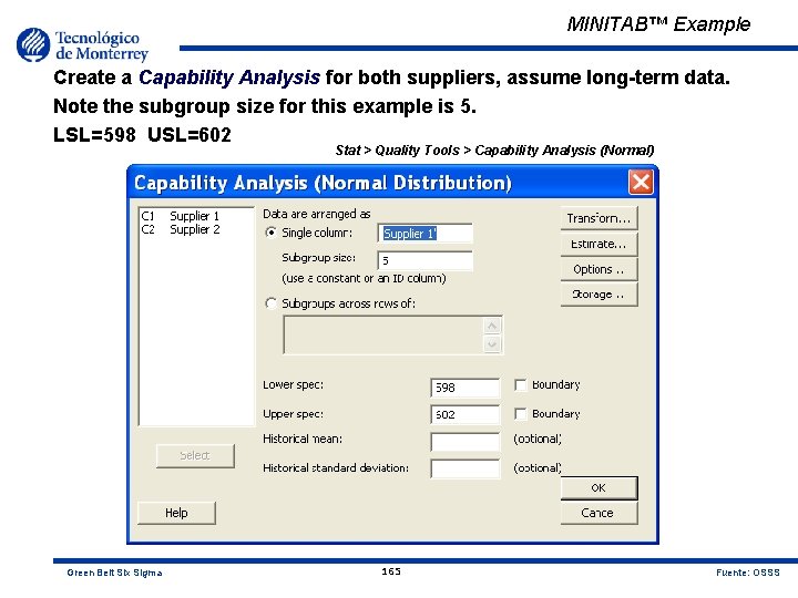
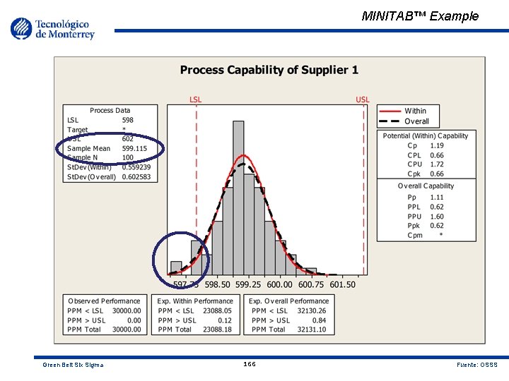
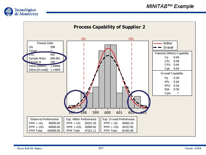
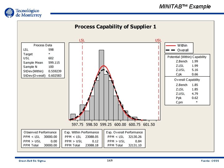
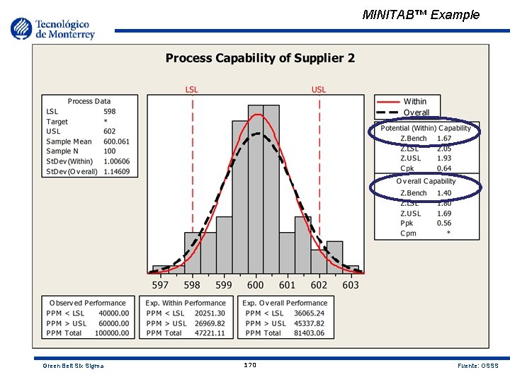
MINITAB™ Example Create a Capability Analysis for both suppliers, assume long-term data. Note the subgroup size for this example is 5. LSL=598 USL=602 Stat > Quality Tools > Capability Analysis (Normal) Green Belt Six Sigma 165 Fuente: OSSS

MINITAB™ Example Green Belt Six Sigma 166 Fuente: OSSS

MINITAB™ Example Green Belt Six Sigma 167 Fuente: OSSS

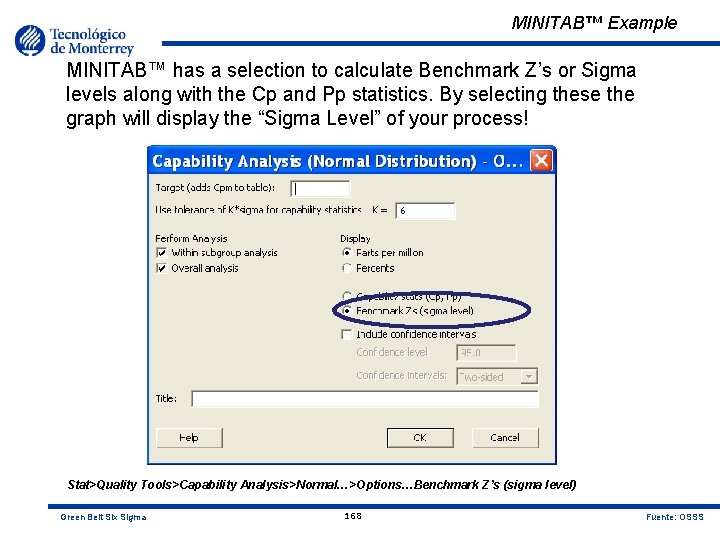
MINITAB™ Example MINITAB™ has a selection to calculate Benchmark Z’s or Sigma levels along with the Cp and Pp statistics. By selecting these the graph will display the “Sigma Level” of your process! Stat>Quality Tools>Capability Analysis>Normal…>Options…Benchmark Z’s (sigma level) Green Belt Six Sigma 168 Fuente: OSSS

MINITAB™ Example Green Belt Six Sigma 169 Fuente: OSSS

MINITAB™ Example Green Belt Six Sigma 170 Fuente: OSSS

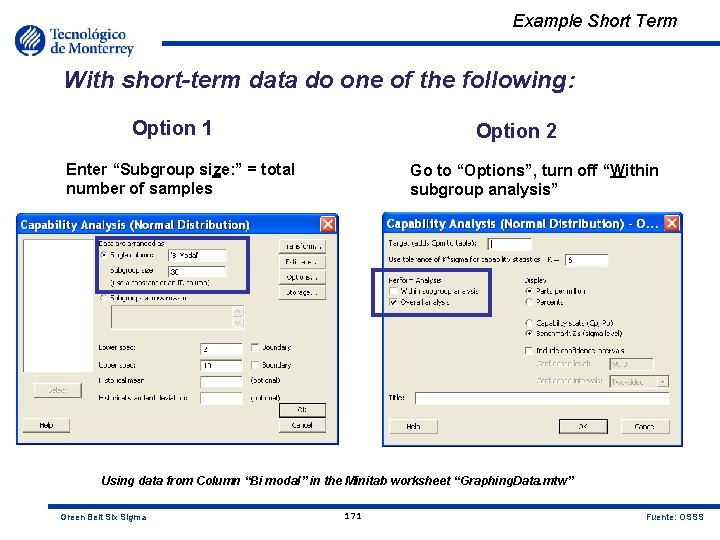
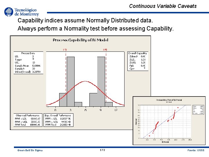
Example Short Term With short-term data do one of the following: Option 1 Option 2 Enter “Subgroup size: ” = total number of samples Go to “Options”, turn off “Within subgroup analysis” Using data from Column “Bi modal” in the Minitab worksheet “Graphing. Data. mtw” Green Belt Six Sigma 171 Fuente: OSSS

Continuous Variable Caveats Capability indices assume Normally Distributed data. Always perform a Normality test before assessing Capability. Green Belt Six Sigma 172 Fuente: OSSS

Capability Steps We can follow the steps for calculating capability for Continuous Data until we reach the question about data Normality… Select Output for Improvement #1 Verify Customer Requirements #2 Validate Specification Limits #3 Collect Sample Data #4 Determine Data Type (LT or ST) #5 Check data for Normality #6 Calculate Z-Score, PPM, Yield, Capability Cp, Cpk, Ppk #7 Green Belt Six Sigma 173 Fuente: OSSS

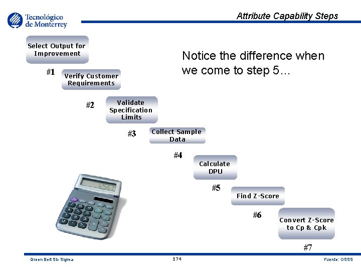
Attribute Capability Steps Select Output for Improvement #1 Notice the difference when we come to step 5… Verify Customer Requirements #2 Validate Specification Limits #3 Collect Sample Data #4 Calculate DPU #5 Find Z-Score #6 Convert Z-Score to Cp & Cpk #7 Green Belt Six Sigma 174 Fuente: OSSS

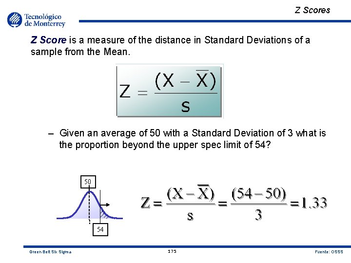
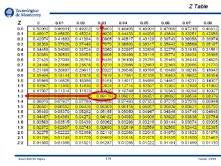
Z Scores Z Score is a measure of the distance in Standard Deviations of a sample from the Mean. – Given an average of 50 with a Standard Deviation of 3 what is the proportion beyond the upper spec limit of 54? 50 54 Green Belt Six Sigma 175 Fuente: OSSS

Z Table Green Belt Six Sigma 176 Fuente: OSSS

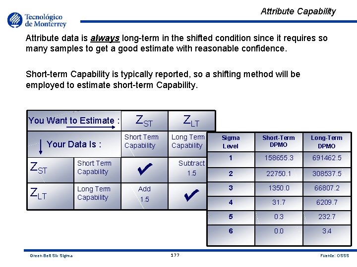
Attribute Capability Attribute data is always long-term in the shifted condition since it requires so many samples to get a good estimate with reasonable confidence. Short-term Capability is typically reported, so a shifting method will be employed to estimate short-term Capability. You Want to Estimate : Your Data Is : ZST Short Term Capability ZLT Long Term Capability Green Belt Six Sigma ZST Short Term Capability ZLT Long Term Capability Subtract 1. 5 Add 1. 5 177 Sigma Level Short-Term DPMO Long-Term DPMO 1 158655. 3 691462. 5 2 22750. 1 308537. 5 3 1350. 0 66807. 2 4 31. 7 6209. 7 5 0. 3 232. 7 6 0. 0 3. 4 Fuente: OSSS

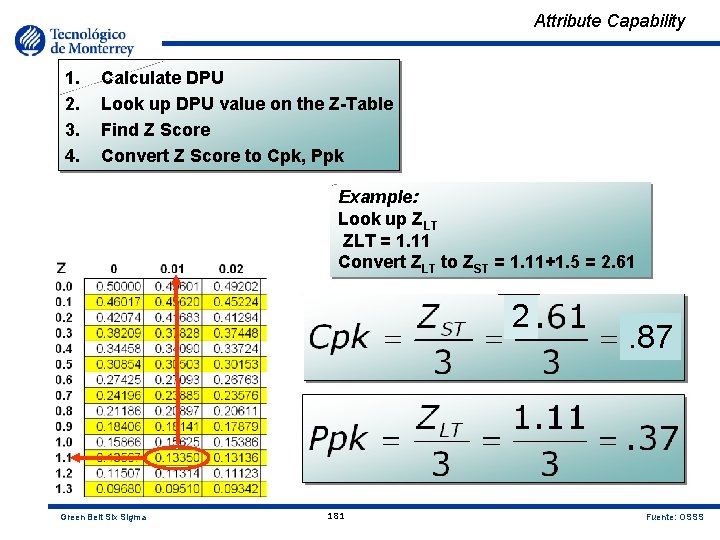
Attribute Capability By viewing these formulas you can see there is a relationship between them. If we divide our Z short-term by 3 we can determine our Cpk and if we divide our Z long-term by 3 we can determine our Ppk. Green Belt Six Sigma 178 Fuente: OSSS

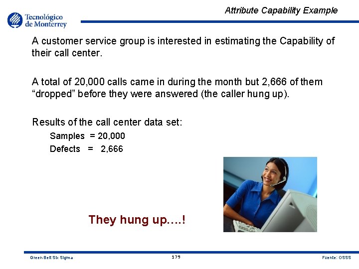
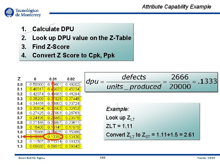
Attribute Capability Example A customer service group is interested in estimating the Capability of their call center. A total of 20, 000 calls came in during the month but 2, 666 of them “dropped” before they were answered (the caller hung up). Results of the call center data set: Samples = 20, 000 Defects = 2, 666 They hung up…. ! Green Belt Six Sigma 179 Fuente: OSSS

Attribute Capability Example 1. 2. 3. 4. Calculate DPU Look up DPU value on the Z-Table Find Z-Score Convert Z Score to Cpk, Ppk Example: Look up ZLT = 1. 11 Convert ZLT to ZST = 1. 11+1. 5 = 2. 61 Green Belt Six Sigma 180 Fuente: OSSS

Attribute Capability 1. 2. 3. 4. Calculate DPU Look up DPU value on the Z-Table Find Z Score Convert Z Score to Cpk, Ppk Example: Look up ZLT = 1. 11 Convert ZLT to ZST = 1. 11+1. 5 = 2. 61 2 Green Belt Six Sigma 181 . 87 Fuente: OSSS

Summary At this point, you should be able to: • Estimate Capability for Continuous Data • Estimate Capability for Attribute Data • Describe the impact of Non-normal Data on the analysis presented in this module for Continuous Capability Green Belt Six Sigma 182 Fuente: OSSS

Measure Phase Wrap Up and Action Items

Measure Phase Overview - The Goal The goal of the Measure Phase is to: • Define, explore and classify “X” variables using a variety of tools. – – Detailed Process Mapping Fishbone Diagrams X-Y Matrixes FMEA • Demonstrate a working knowledge of Basic Statistics to use as a communication tool and a basis for inference. • Perform Measurement Capability studies on output variables. • Evaluate stability of process and estimate starting point capability. Green Belt Six Sigma 184 Fuente: OSSS

Six Sigma Behaviors • Being tenacious, courageous • Being rigorous, disciplined • Making data-based decisions • Embracing change & continuous learning Walk the Walk! • Sharing best practices Each “player” in the Six Sigma process must be A ROLE MODEL for the Lean Six Sigma culture Green Belt Six Sigma 185 Fuente: OSSS

Measure Phase Deliverables Listed here are the Measure Deliverables that each candidate should present in a Power Point presentation to their mentor and project champion. At this point you should understand what is necessary to provide these deliverables in your presentation. – – – Team Members (Team Meeting Attendance) Primary Metric Secondary Metric(s) Process Map – detailed FMEA X-Y Matrix Basic Statistics on Y MSA Stability graphs Capability Analysis Project Plan Issues and Barriers Green Belt Six Sigma 186 Fuente: OSSS

Measure Phase - The Roadblocks Look for the potential roadblocks and plan to address them before they become problems: – Team members do not have the time to collect data. – Data presented is the best guess by functional managers. – Process participants do not participate in the creation of the X-Y Matrix, FMEA and Process Map. It won’t all be smooth sailing…. . Green Belt Six Sigma 187 Fuente: OSSS

Champion/ Process Owner DMAIC Roadmap Identify Problem Area Define Determine Appropriate Project Focus Estimate COPQ Improve Analyze Measure Establish Team Assess Stability, Capability, and Measurement Systems Identify and Prioritize All X’s Prove/Disprove Impact X’s Have On Problem Identify, Prioritize, Select Solutions Control or Eliminate X ’s Causing Problems Control Implement Solutions to Control or Eliminate X ’s Causing Problems Implement Control Plan to Ensure Problem Doesn ’t Return Verify Financial Impact Green Belt Six Sigma 188 Fuente: OSSS

Measure Phase Detailed Problem Statement Determined Detailed Process Mapping Identify All Process X’s Causing Problems (Fishbone, Process Map) Select the Vital Few X’s Causing Problems (X-Y Matrix, FMEA) Assess Measurement System N Repeatable & Reproducible? Y Implement Changes to Make System Acceptable Assess Stability (Statistical Control) Assess Capability (Problem with Centering/Spread) Estimate Process Sigma Level Review Progress with Champion Ready for Analyze Green Belt Six Sigma 189 Fuente: OSSS

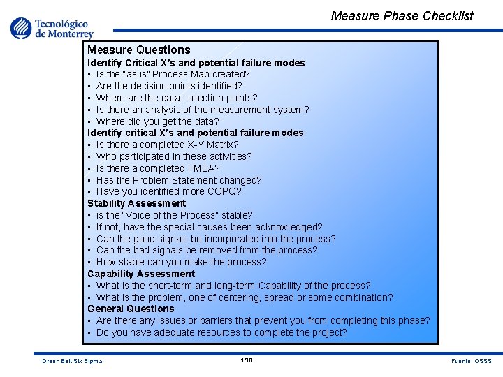
Measure Phase Checklist Measure Questions Identify Critical X’s and potential failure modes • Is the “as is” Process Map created? • Are the decision points identified? • Where are the data collection points? • Is there an analysis of the measurement system? • Where did you get the data? Identify critical X’s and potential failure modes • Is there a completed X-Y Matrix? • Who participated in these activities? • Is there a completed FMEA? • Has the Problem Statement changed? • Have you identified more COPQ? Stability Assessment • is the “Voice of the Process” stable? • If not, have the special causes been acknowledged? • Can the good signals be incorporated into the process? • Can the bad signals be removed from the process? • How stable can you make the process? Capability Assessment • What is the short-term and long-term Capability of the process? • What is the problem, one of centering, spread or some combination? General Questions • Are there any issues or barriers that prevent you from completing this phase? • Do you have adequate resources to complete the project? Green Belt Six Sigma 190 Fuente: OSSS

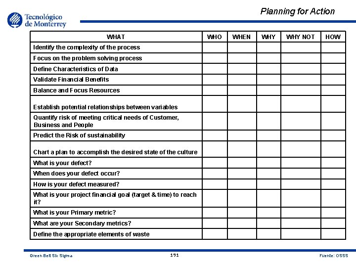
Planning for Action WHAT WHO WHEN WHY NOT HOW Identify the complexity of the process Focus on the problem solving process Define Characteristics of Data Validate Financial Benefits Balance and Focus Resources Establish potential relationships between variables Quantify risk of meeting critical needs of Customer, Business and People Predict the Risk of sustainability Chart a plan to accomplish the desired state of the culture What is your defect? When does your defect occur? How is your defect measured? What is your project financial goal (target & time) to reach it? What is your Primary metric? What are your Secondary metrics? Define the appropriate elements of waste Green Belt Six Sigma 191 Fuente: OSSS

Summary At this point, you should: • Have a clear understanding of the specific action items • Have started to develop a project plan to complete the action items • Have identified ways to deal with potential roadblocks • Be ready to apply the Six Sigma method within your business Green Belt Six Sigma 192 Fuente: OSSS