GPCA Generalized Principal Component Analysis Theory and Applications

GPCA Generalized Principal Component Analysis: Theory and Applications in Vision & Control René Vidal Center for Imaging Science Johns Hopkins University

Outline n Motivation: convergence of vision, learning and robotics n Part I: Generalized Principal Component Analysis (1 h) n n Principal Component Analysis (PCA) and extensions Representing multiple subspaces as algebraic varieties Segmenting subspaces by polynomial fitting & differentiation Applications: n n Part II: Reconstruction of Dynamic Scenes (1 h) n n n image segmentation/compression, face recognition 2 -D and 3 -D motion segmentation Segmentation of dynamic textures MRI-based heart motion analysis DTI-based spinal cord injury detection Part III: Identification of Hybrid Systems (30 min) Copyright @ Rene Vidal 2

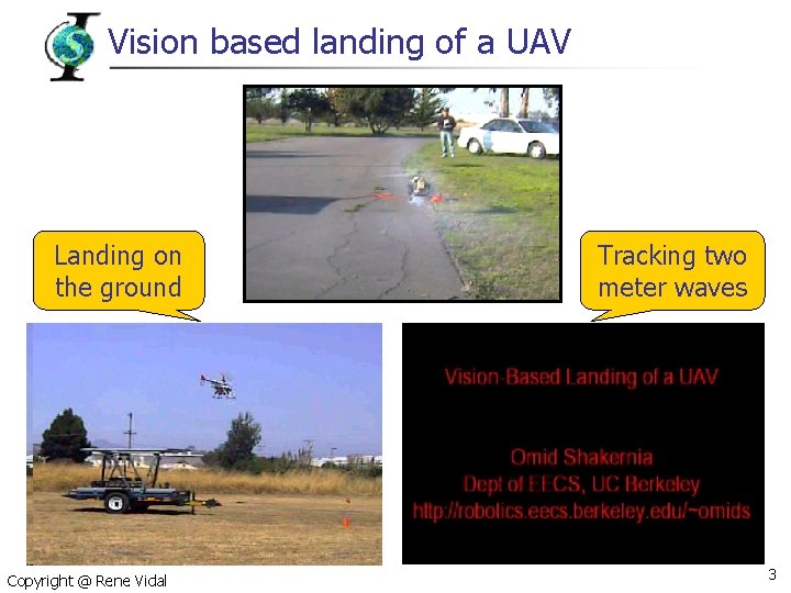
Vision based landing of a UAV Landing on the ground Copyright @ Rene Vidal Tracking two meter waves 3

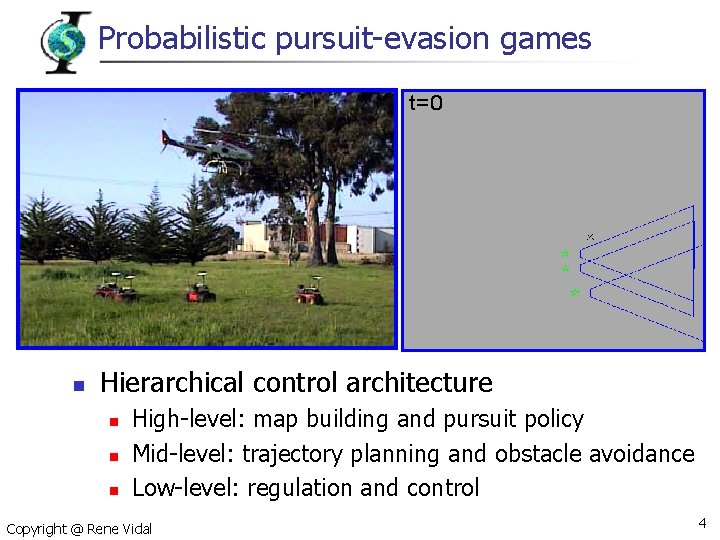
Probabilistic pursuit-evasion games n Hierarchical control architecture n n n High-level: map building and pursuit policy Mid-level: trajectory planning and obstacle avoidance Low-level: regulation and control Copyright @ Rene Vidal 4

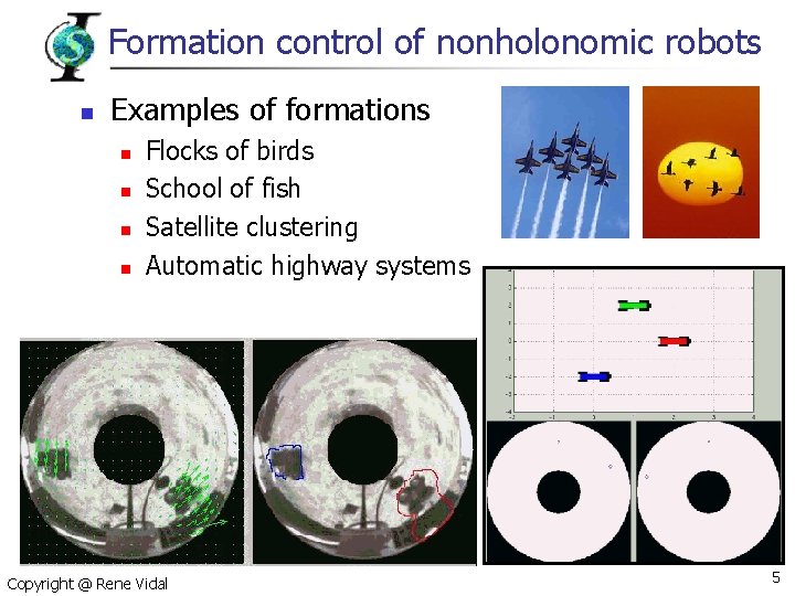
Formation control of nonholonomic robots n Examples of formations n n Flocks of birds School of fish Satellite clustering Automatic highway systems Copyright @ Rene Vidal 5

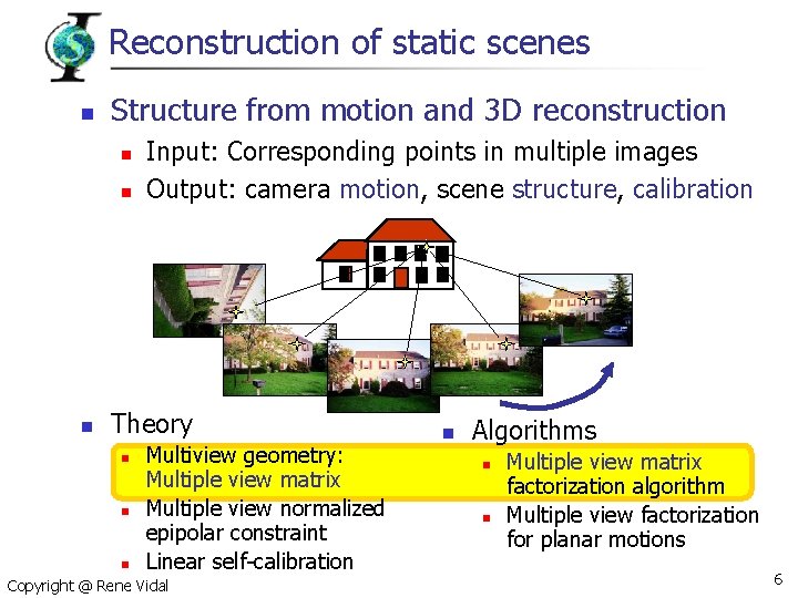
Reconstruction of static scenes n Structure from motion and 3 D reconstruction n Input: Corresponding points in multiple images Output: camera motion, scene structure, calibration Theory n n n Multiview geometry: Multiple view matrix Multiple view normalized epipolar constraint Linear self-calibration Copyright @ Rene Vidal n Algorithms n n Multiple view matrix factorization algorithm Multiple view factorization for planar motions 6

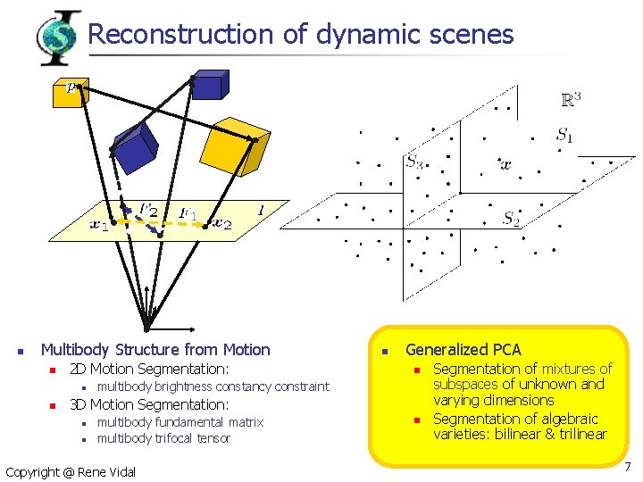
Reconstruction of dynamic scenes n Multibody Structure from Motion n 2 D Motion Segmentation: n n n Generalized PCA n multibody brightness constancy constraint 3 D Motion Segmentation: n n multibody fundamental matrix multibody trifocal tensor Copyright @ Rene Vidal n Segmentation of mixtures of subspaces of unknown and varying dimensions Segmentation of algebraic varieties: bilinear & trilinear 7

Part I: Generalized Principal Component Analysis René Vidal Center for Imaging Science Johns Hopkins University

Principal Component Analysis (PCA) n n Applications: data compression, regression, image analysis (eigenfaces), pattern recognition Identify a linear subspace S from sample points Basis for S Copyright @ Rene Vidal 9

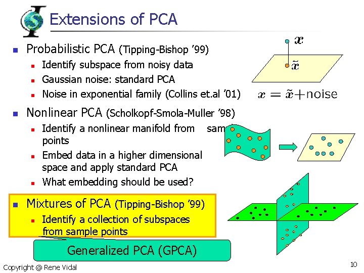
Extensions of PCA n Probabilistic PCA (Tipping-Bishop ’ 99) n n Nonlinear PCA (Scholkopf-Smola-Muller ’ 98) n n Identify subspace from noisy data Gaussian noise: standard PCA Noise in exponential family (Collins et. al ’ 01) Identify a nonlinear manifold from sample points Embed data in a higher dimensional space and apply standard PCA What embedding should be used? Mixtures of PCA (Tipping-Bishop ’ 99) n Identify a collection of subspaces from sample points Generalized PCA (GPCA) Copyright @ Rene Vidal 10

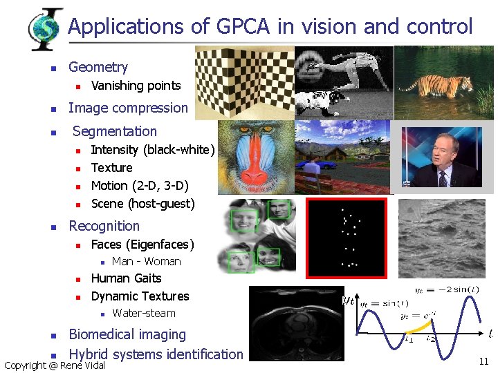
Applications of GPCA in vision and control n Geometry n n n Image compression Segmentation n n Vanishing points Intensity (black-white) Texture Motion (2 -D, 3 -D) Scene (host-guest) Recognition n Faces (Eigenfaces) n n n Human Gaits Dynamic Textures n n n Man - Woman Water-steam Biomedical imaging Hybrid systems identification Copyright @ Rene Vidal 11

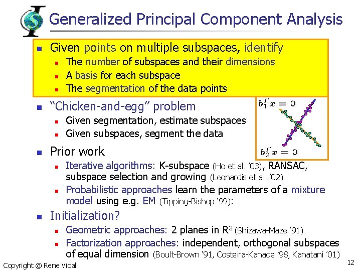
Generalized Principal Component Analysis n Given points on multiple subspaces, identify n n “Chicken-and-egg” problem n n n Given segmentation, estimate subspaces Given subspaces, segment the data Prior work n n n The number of subspaces and their dimensions A basis for each subspace The segmentation of the data points Iterative algorithms: K-subspace (Ho et al. ’ 03), RANSAC, subspace selection and growing (Leonardis et al. ’ 02) Probabilistic approaches learn the parameters of a mixture model using e. g. EM (Tipping-Bishop ‘ 99): Initialization? n n Geometric approaches: 2 planes in R 3 (Shizawa-Maze ’ 91) Factorization approaches: independent, orthogonal subspaces of equal dimension (Boult-Brown ‘ 91, Costeira-Kanade ‘ 98, Kanatani ’ 01) Copyright @ Rene Vidal 12

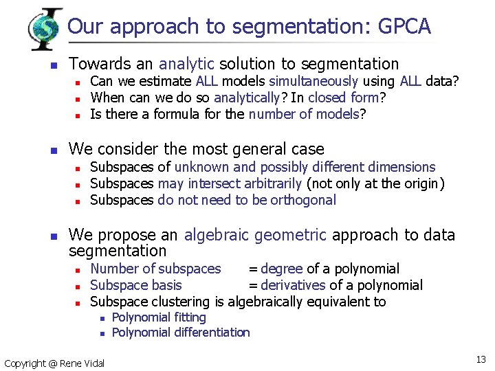
Our approach to segmentation: GPCA n Towards an analytic solution to segmentation n n We consider the most general case n n Can we estimate ALL models simultaneously using ALL data? When can we do so analytically? In closed form? Is there a formula for the number of models? Subspaces of unknown and possibly different dimensions Subspaces may intersect arbitrarily (not only at the origin) Subspaces do not need to be orthogonal We propose an algebraic geometric approach to data segmentation n Number of subspaces = degree of a polynomial Subspace basis = derivatives of a polynomial Subspace clustering is algebraically equivalent to n n Copyright @ Rene Vidal Polynomial fitting Polynomial differentiation 13

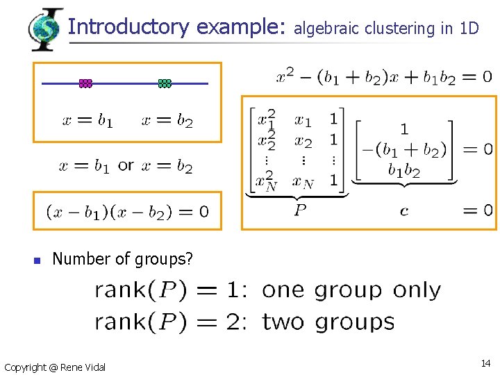
Introductory example: n algebraic clustering in 1 D Number of groups? Copyright @ Rene Vidal 14

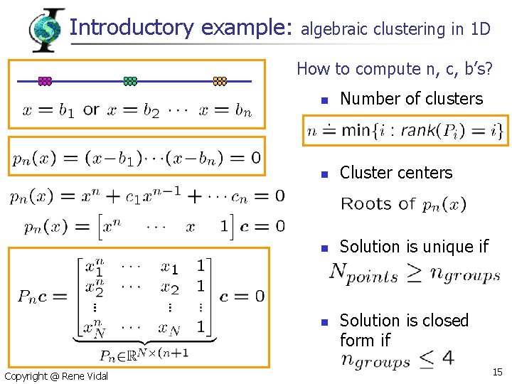
Introductory example: algebraic clustering in 1 D How to compute n, c, b’s? n Number of clusters n Cluster centers n Solution is unique if n Copyright @ Rene Vidal Solution is closed form if 15

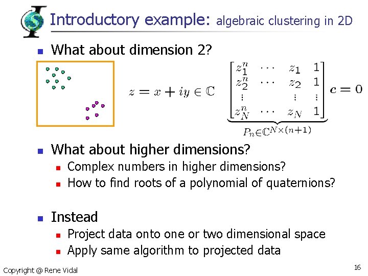
Introductory example: algebraic clustering in 2 D n What about dimension 2? n What about higher dimensions? n n n Complex numbers in higher dimensions? How to find roots of a polynomial of quaternions? Instead n n Project data onto one or two dimensional space Apply same algorithm to projected data Copyright @ Rene Vidal 16

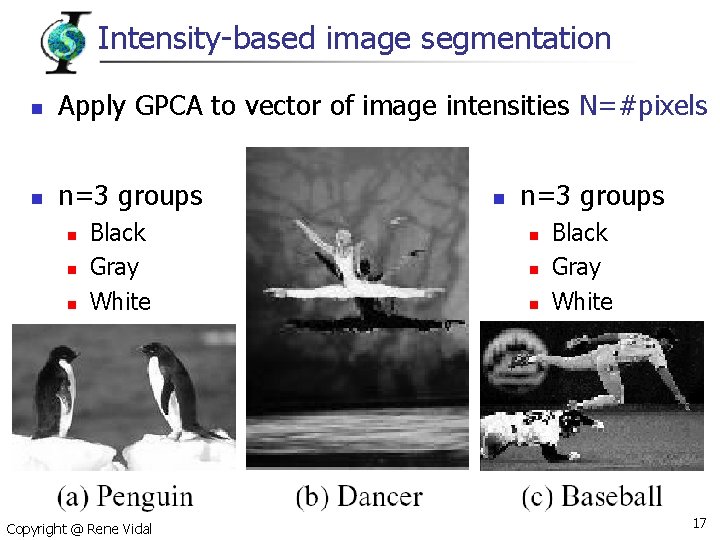
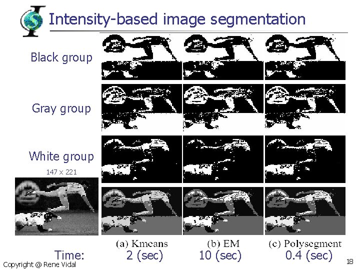
Intensity-based image segmentation n Apply GPCA to vector of image intensities N=#pixels n n=3 groups n n n Black Gray White Copyright @ Rene Vidal n n=3 groups n n n Black Gray White 17

Intensity-based image segmentation Black group Gray group White group 147 x 221 Time: Copyright @ Rene Vidal 2 (sec) 10 (sec) 0. 4 (sec) 18

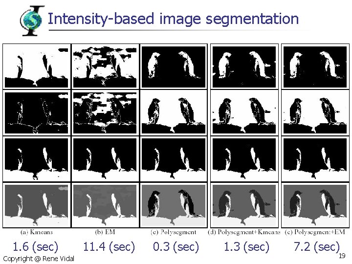
Intensity-based image segmentation 1. 6 (sec) Copyright @ Rene Vidal 11. 4 (sec) 0. 3 (sec) 1. 3 (sec) 7. 2 (sec) 19

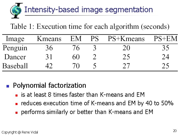
Intensity-based image segmentation n Polynomial factorization n is at least 8 times faster than K-means and EM reduces execution time of K-means and EM by 40 to 50% performs similarly or better than K-means and EM Copyright @ Rene Vidal 20

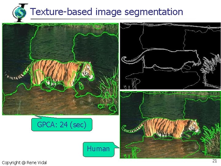
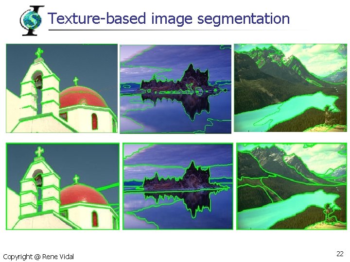
Texture-based image segmentation GPCA: 24 (sec) Human Copyright @ Rene Vidal 21

Texture-based image segmentation Copyright @ Rene Vidal 22

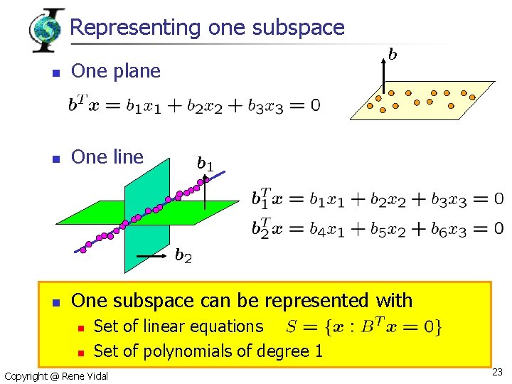
Representing one subspace n One plane n One line n One subspace can be represented with n n Set of linear equations Set of polynomials of degree 1 Copyright @ Rene Vidal 23

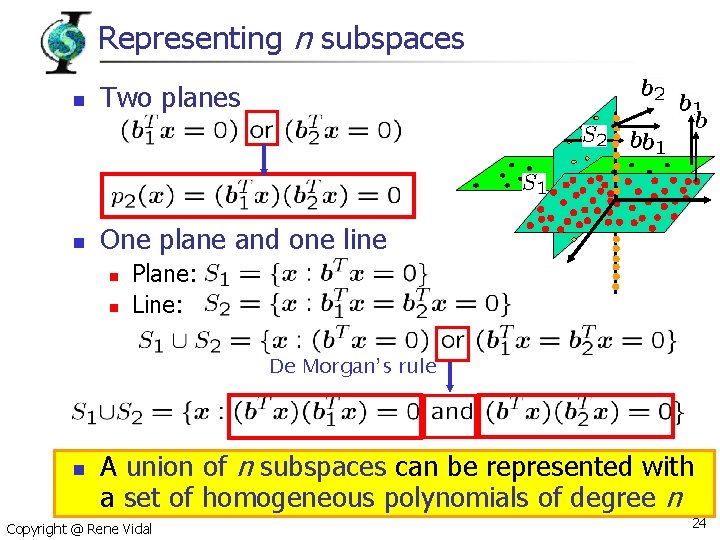
Representing n subspaces n Two planes n One plane and one line n n Plane: Line: De Morgan’s rule n A union of n subspaces can be represented with a set of homogeneous polynomials of degree n Copyright @ Rene Vidal 24

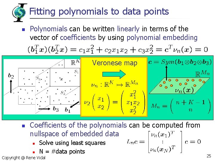
Fitting polynomials to data points n Polynomials can be written linearly in terms of the vector of coefficients by using polynomial embedding Veronese map n Coefficients of the polynomials can be computed from nullspace of embedded data n n Solve using least squares N = #data points Copyright @ Rene Vidal 25

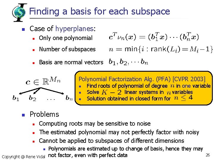
Finding a basis for each subspace n Case of hyperplanes: n Only one polynomial n Number of subspaces n Basis are normal vectors Polynomial Factorization Alg. (PFA) [CVPR 2003] n n Find roots of polynomial of degree in one variable Solve linear systems in variables Solution obtained in closed form for Problems n n n Computing roots may be sensitive to noise The estimated polynomial may not perfectly factor with noisy Cannot be applied to subspaces of different dimensions n Copyright @ Rene Vidal Polynomials are estimated up to change of basis, hence they may not factor, even with perfect data 26

Finding a basis for each subspace Theorem: GPCA by differentiation n To learn a mixture of subspaces we just need one positive example per class Copyright @ Rene Vidal 27

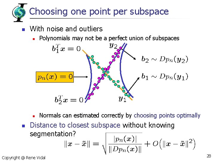
Choosing one point per subspace n n With noise and outliers n Polynomials may not be a perfect union of subspaces n Normals can estimated correctly by choosing points optimally Distance to closest subspace without knowing segmentation? Copyright @ Rene Vidal 28

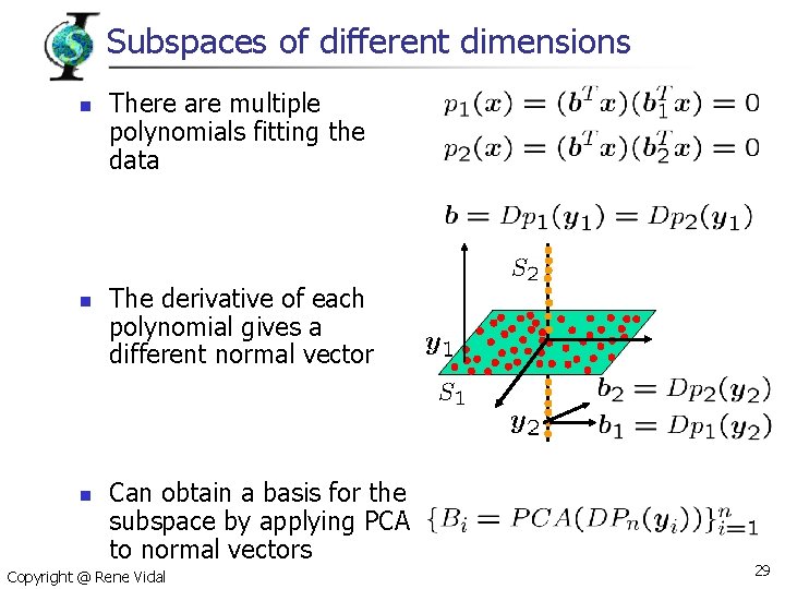
Subspaces of different dimensions n n n There are multiple polynomials fitting the data The derivative of each polynomial gives a different normal vector Can obtain a basis for the subspace by applying PCA to normal vectors Copyright @ Rene Vidal 29

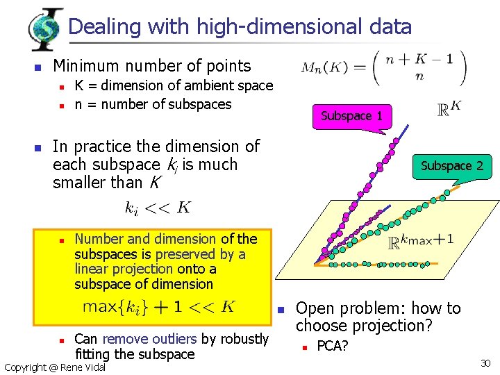
Dealing with high-dimensional data n Minimum number of points n n n K = dimension of ambient space n = number of subspaces Subspace 1 In practice the dimension of each subspace ki is much smaller than K n Subspace 2 Number and dimension of the subspaces is preserved by a linear projection onto a subspace of dimension n n Can remove outliers by robustly fitting the subspace Copyright @ Rene Vidal Open problem: how to choose projection? n PCA? 30

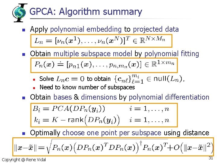
GPCA: Algorithm summary n Apply polynomial embedding to projected data n Obtain multiple subspace model by polynomial fitting n n Solve to obtain Need to know number of subspaces n Obtain bases & dimensions by polynomial differentiation n Optimally choose one point per subspace using distance Copyright @ Rene Vidal 31

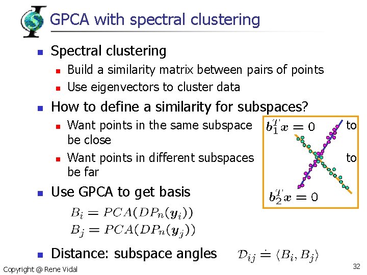
GPCA with spectral clustering n Spectral clustering n n n Build a similarity matrix between pairs of points Use eigenvectors to cluster data How to define a similarity for subspaces? n n Want points in the same subspace be close Want points in different subspaces be far n Use GPCA to get basis n Distance: subspace angles Copyright @ Rene Vidal to to 32

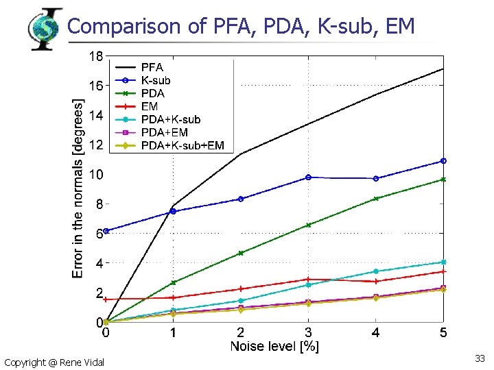
Comparison of PFA, PDA, K-sub, EM Copyright @ Rene Vidal 33

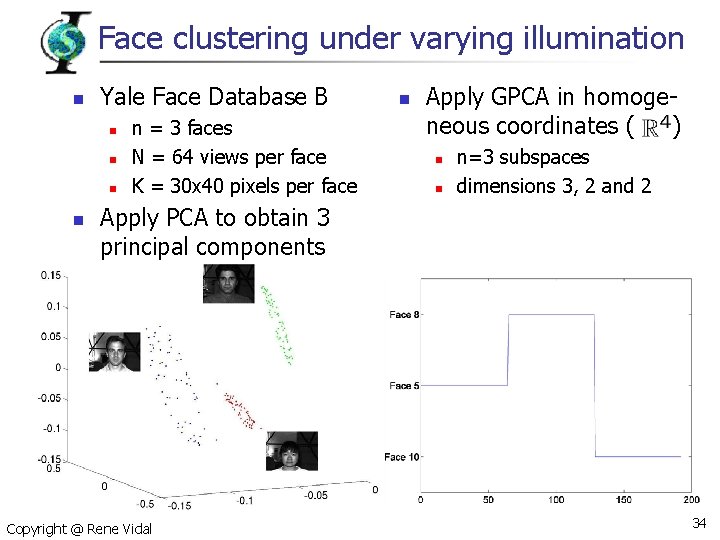
Face clustering under varying illumination n Yale Face Database B n n n = 3 faces N = 64 views per face K = 30 x 40 pixels per face n Apply GPCA in homogeneous coordinates ( ) n n n=3 subspaces dimensions 3, 2 and 2 Apply PCA to obtain 3 principal components Copyright @ Rene Vidal 34

Summary n GPCA: algorithm for clustering subspaces n n n Our approach is based on n n Deals with unknown and possibly different dimensions Deals with arbitrary intersections among the subspaces Projecting data onto a low-dimensional subspace Fitting polynomials to projected subspaces Differentiating polynomials to obtain a basis Applications in image processing and computer vision n Image segmentation: intensity and texture Image compression Face recognition under varying illumination Copyright @ Rene Vidal 35

Part II Reconstruction of Dynamic Scenes René Vidal Center for Imaging Science Johns Hopkins University

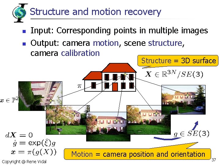
Structure and motion recovery n n Input: Corresponding points in multiple images Output: camera motion, scene structure, camera calibration Structure = 3 D surface Motion = camera position and orientation Copyright @ Rene Vidal 37

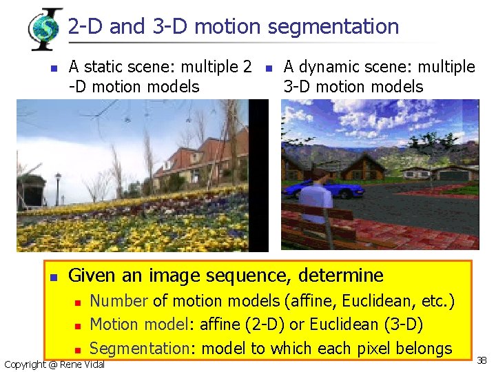
2 -D and 3 -D motion segmentation n n A static scene: multiple 2 -D motion models n A dynamic scene: multiple 3 -D motion models Given an image sequence, determine n n Number of motion models (affine, Euclidean, etc. ) Motion model: affine (2 -D) or Euclidean (3 -D) Segmentation: model to which each pixel belongs n Copyright @ Rene Vidal 38

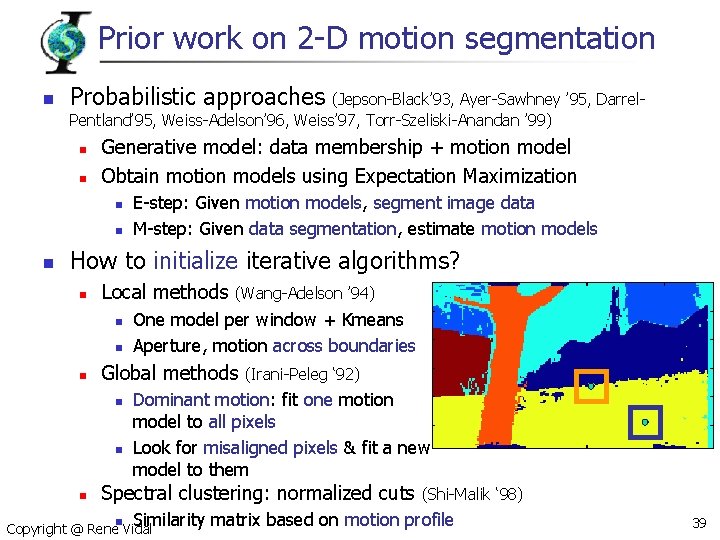
Prior work on 2 -D motion segmentation n Probabilistic approaches (Jepson-Black’ 93, Ayer-Sawhney ’ 95, Darrel. Pentland’ 95, Weiss-Adelson’ 96, Weiss’ 97, Torr-Szeliski-Anandan ’ 99) n n Generative model: data membership + motion model Obtain motion models using Expectation Maximization n E-step: Given motion models, segment image data M-step: Given data segmentation, estimate motion models How to initialize iterative algorithms? n Local methods n n n One model per window + Kmeans Aperture, motion across boundaries Global methods n n n (Wang-Adelson ’ 94) (Irani-Peleg ‘ 92) Dominant motion: fit one motion model to all pixels Look for misaligned pixels & fit a new model to them Spectral clustering: normalized cuts n (Shi-Malik ‘ 98) Similarity matrix based on motion profile Copyright @ Rene Vidal 39

Prior work on 3 -D motion segmentation n Affine cameras, multiple views n n (Costeira-Kanade ’ 98, Gear ’ 98, Han. Kanade ’ 01, Kanatani ’ 01 -02, Han-Kanade ‘ 00) Perspective cameras (statistical approaches) n n n Factorization methods: Motion segmentation & model selection (Torr’ 98) Multiple rigid motions using NCuts+EM (Feng-Perona ’ 98) Perspective cameras (geometric approaches) n n n Points in a line (Shashua-Levin ‘ 01) Points in a plane moving linearly at constant speed Points in moving in planes (Sturm ’ 02) Segmentation of two rigid motions (Wolf-Shashua ‘ 01) n Copyright @ Rene Vidal 40

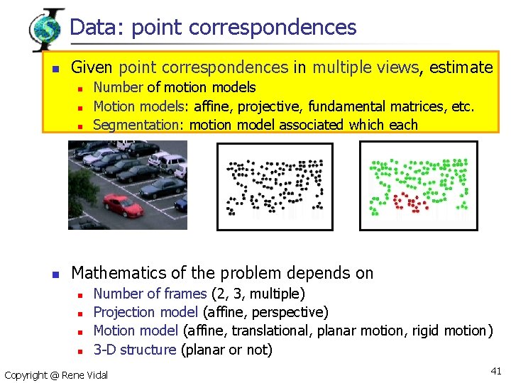
Data: point correspondences n Given point correspondences in multiple views, estimate n n Number of motion models Motion models: affine, projective, fundamental matrices, etc. Segmentation: motion model associated which each Mathematics of the problem depends on n n Number of frames (2, 3, multiple) Projection model (affine, perspective) Motion model (affine, translational, planar motion, rigid motion) 3 -D structure (planar or not) Copyright @ Rene Vidal 41

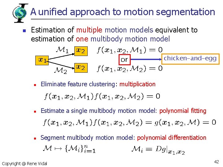
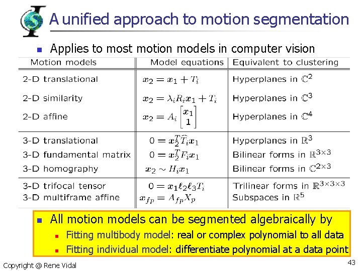
A unified approach to motion segmentation n Estimation of multiple motion models equivalent to estimation of one multibody motion model chicken-and-egg n Eliminate feature clustering: multiplication n Estimate a single multibody motion model: polynomial fitting n Segment multibody motion model: polynomial differentiation Copyright @ Rene Vidal 42

A unified approach to motion segmentation n Applies to most motion models in computer vision n All motion models can be segmented algebraically by n n Fitting multibody model: real or complex polynomial to all data Fitting individual model: differentiate polynomial at a data point Copyright @ Rene Vidal 43

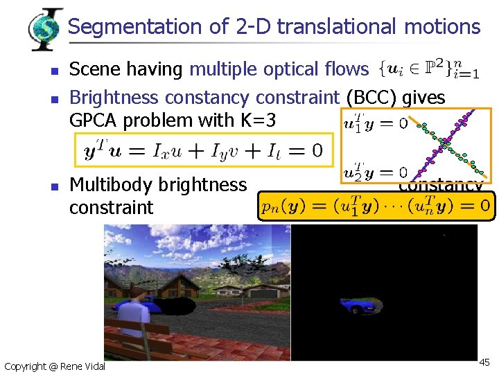
Segmentation of 2 -D translational motions n n n Scene having multiple optical flows Brightness constancy constraint (BCC) gives GPCA problem with K=3 Multibody brightness constraint Copyright @ Rene Vidal constancy 45

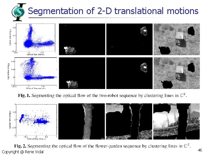
Segmentation of 2 -D translational motions Copyright @ Rene Vidal 46

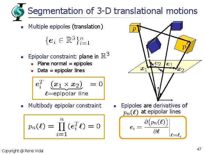
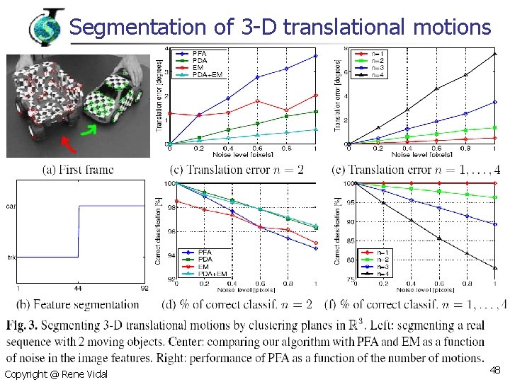
Segmentation of 3 -D translational motions n Multiple epipoles (translation) n Epipolar constraint: plane in n Plane normal = epipoles Data = epipolar lines Multibody epipolar constraint Copyright @ Rene Vidal n Epipoles are derivatives of at epipolar lines 47

Segmentation of 3 -D translational motions Copyright @ Rene Vidal 48

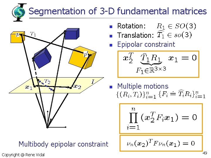
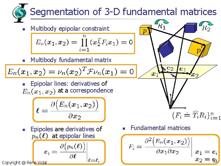
Segmentation of 3 -D fundamental matrices n Rotation: Translation: Epipolar constraint n Multiple motions n n Multibody epipolar constraint Copyright @ Rene Vidal 49

Segmentation of 3 -D fundamental matrices n Multibody epipolar constraint n Multibody fundamental matrix n n Epipolar lines: derivatives of at a correspondence Epipoles are derivatives of at epipolar lines Copyright @ Rene Vidal n Fundamental matrices 50

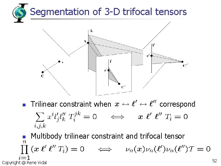
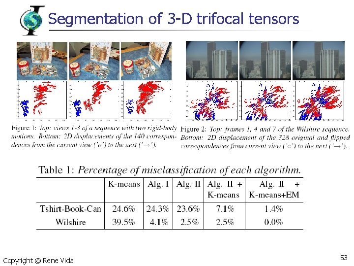
Segmentation of 3 -D trifocal tensors n Trilinear constraint when n Multibody trilinear constraint and trifocal tensor Copyright @ Rene Vidal correspond 52

Segmentation of 3 -D trifocal tensors Copyright @ Rene Vidal 53

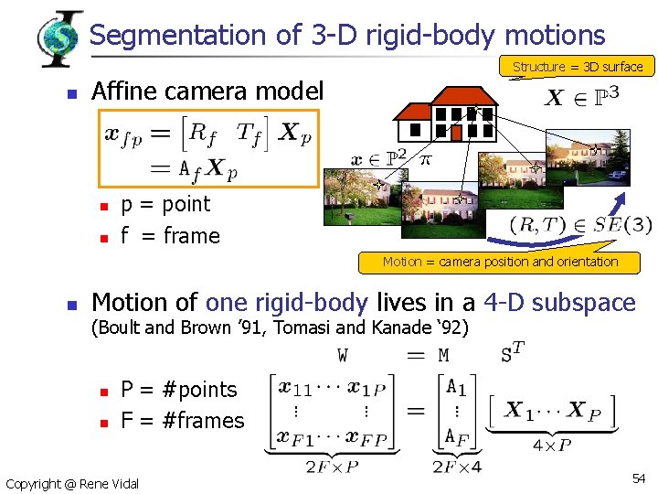
Segmentation of 3 -D rigid-body motions Structure = 3 D surface n Affine camera model n n p = point f = frame Motion = camera position and orientation n Motion of one rigid-body lives in a 4 -D subspace (Boult and Brown ’ 91, Tomasi and Kanade ‘ 92) n n P = #points F = #frames Copyright @ Rene Vidal 54

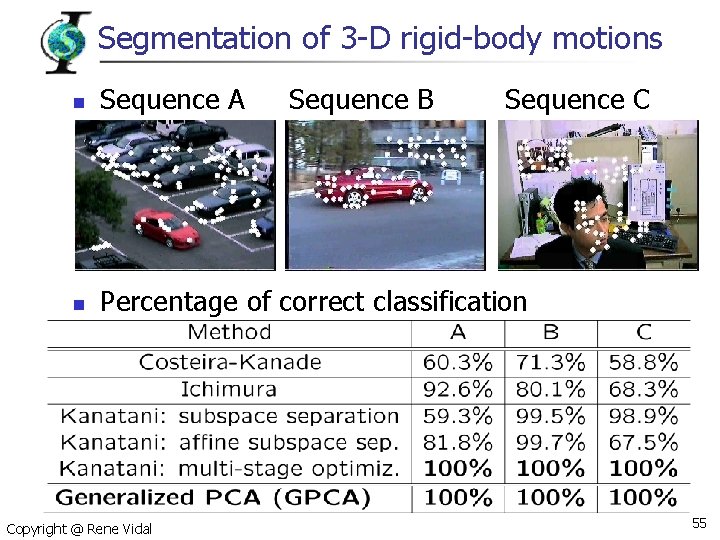
Segmentation of 3 -D rigid-body motions n Sequence A n Percentage of correct classification Copyright @ Rene Vidal Sequence B Sequence C 55

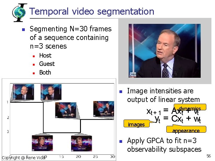
Temporal video segmentation n Segmenting N=30 frames of a sequence containing n=3 scenes n n n Host Guest Both n Image intensities are output of linear system images n Copyright @ Rene Vidal xt + 1 = Axdynamics t + vt yt = Cxt + wt appearance Apply GPCA to fit n=3 observability subspaces 56

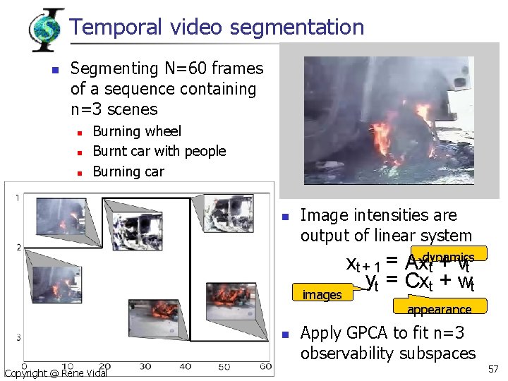
Temporal video segmentation n Segmenting N=60 frames of a sequence containing n=3 scenes n n n Burning wheel Burnt car with people Burning car n Image intensities are output of linear system images n Copyright @ Rene Vidal xt + 1 = Axdynamics t + vt yt = Cxt + wt appearance Apply GPCA to fit n=3 observability subspaces 57

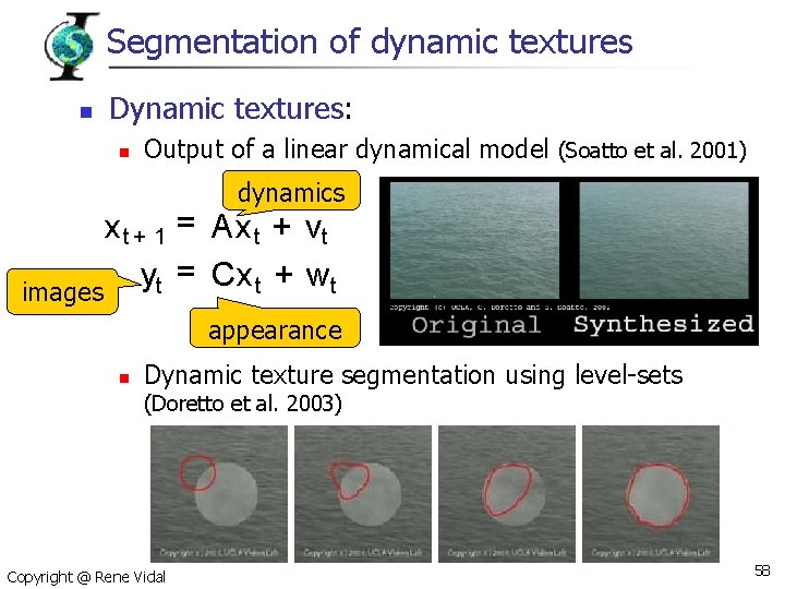
Segmentation of dynamic textures n Dynamic textures: n Output of a linear dynamical model (Soatto et al. 2001) dynamics x t + 1 = Ax t + vt = Cx t + wt y t images appearance n Dynamic texture segmentation using level-sets (Doretto et al. 2003) Copyright @ Rene Vidal 58

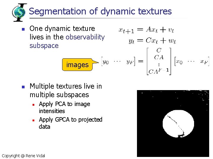
Segmentation of dynamic textures n One dynamic texture lives in the observability subspace images n Multiple textures live in multiple subspaces n n Apply PCA to image intensities Apply GPCA to projected data Copyright @ Rene Vidal 59

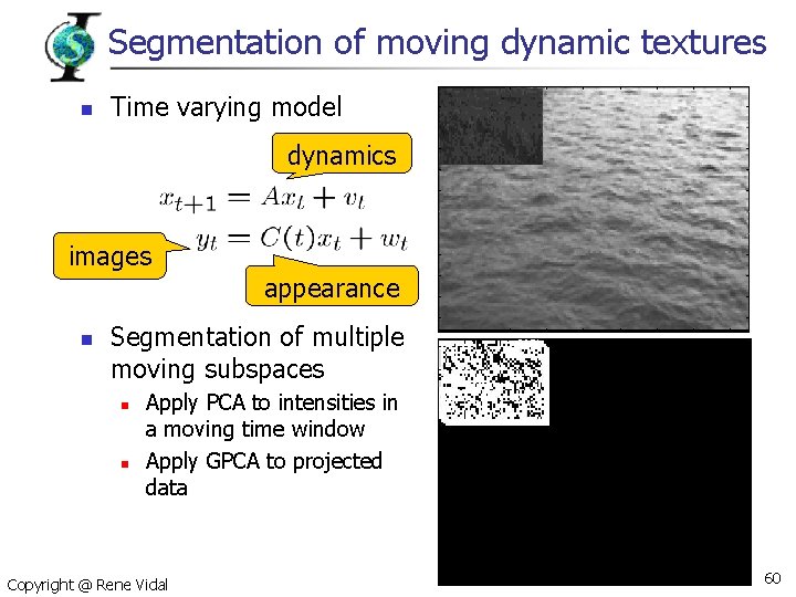
Segmentation of moving dynamic textures n Time varying model dynamics images appearance n Segmentation of multiple moving subspaces n n Apply PCA to intensities in a moving time window Apply GPCA to projected data Copyright @ Rene Vidal 60

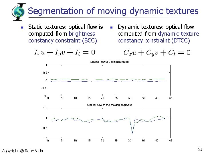
Segmentation of moving dynamic textures n Static textures: optical flow is computed from brightness constancy constraint (BCC) Copyright @ Rene Vidal n Dynamic textures: optical flow computed from dynamic texture constancy constraint (DTCC) 61

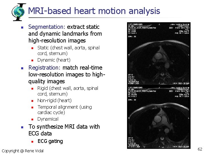
MRI-based heart motion analysis n Segmentation: extract static and dynamic landmarks from high-resolution images n n n Registration: match real-time low-resolution images to highquality images n n n Static (chest wall, aorta, spinal cord, sternum) Dynamic (heart) Rigid (chest wall, aorta, spinal cord, sternum) Non-rigid (heart) Temporal alignment (using cardiac cycle) Dynamical To synthesize MRI data with ECG data n ECG gating Copyright @ Rene Vidal 62

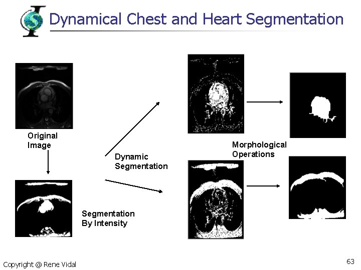
Dynamical Chest and Heart Segmentation Original Image Dynamic Segmentation Morphological Operations Segmentation By Intensity Copyright @ Rene Vidal 63

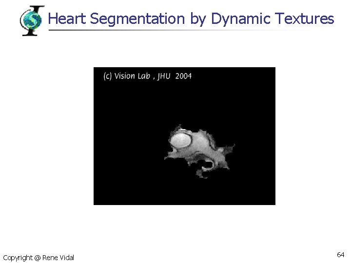
Heart Segmentation by Dynamic Textures Copyright @ Rene Vidal 64

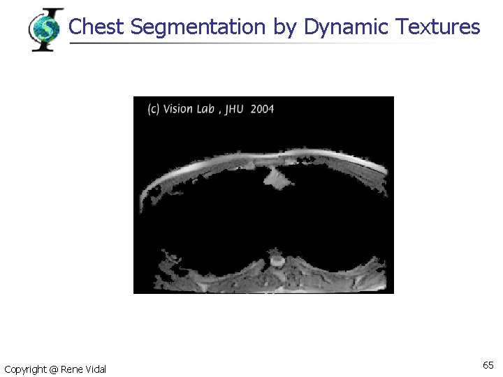
Chest Segmentation by Dynamic Textures Copyright @ Rene Vidal 65

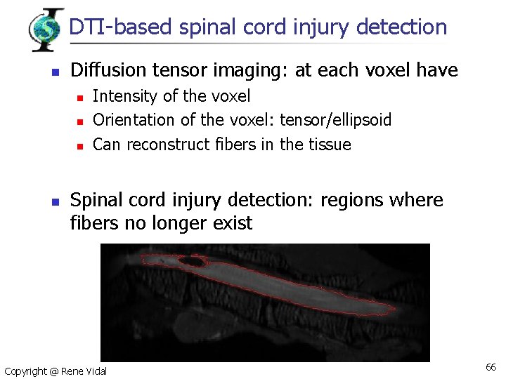
DTI-based spinal cord injury detection n Diffusion tensor imaging: at each voxel have n n Intensity of the voxel Orientation of the voxel: tensor/ellipsoid Can reconstruct fibers in the tissue Spinal cord injury detection: regions where fibers no longer exist Copyright @ Rene Vidal 66

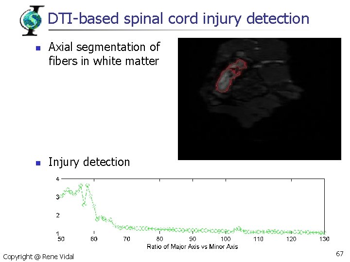
DTI-based spinal cord injury detection n n Axial segmentation of fibers in white matter Injury detection Copyright @ Rene Vidal 67

Conclusions n GPCA gives a unified algebraic approach for the analysis of dynamic scenes n n n Fit a polynomial to all image data Differentiate the polynomial to obtain motion parameters Applies to most motion segmentation problems in vision n Two views n n Three views n Multibody trifocal tensor Multiple views n n 2 -D: translational, similarity, affine 3 -D: translational, fundamental matrices, homographies Affine cameras Open problems n n n Multiple views perspective and central panoramic Dealing with noise (bilinear and trilinear models) Dealing with outliers (all models) Copyright @ Rene Vidal 68

Part III Identification of Hybrid Systems René Vidal Center for Imaging Science Johns Hopkins University

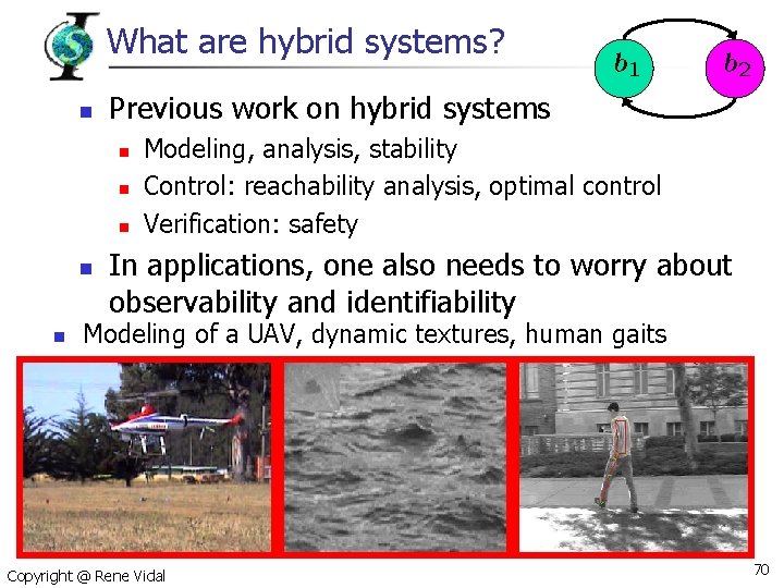
What are hybrid systems? n Previous work on hybrid systems n n n Modeling, analysis, stability Control: reachability analysis, optimal control Verification: safety In applications, one also needs to worry about observability and identifiability Modeling of a UAV, dynamic textures, human gaits Copyright @ Rene Vidal 70

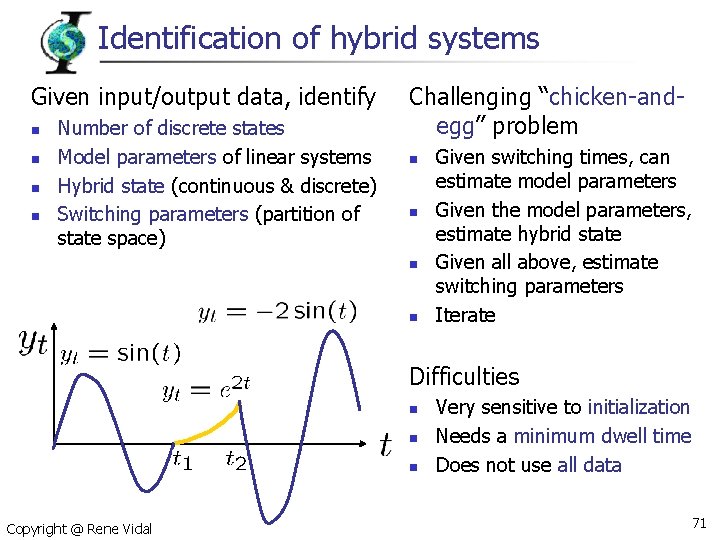
Identification of hybrid systems Given input/output data, identify n n Number of discrete states Model parameters of linear systems Hybrid state (continuous & discrete) Switching parameters (partition of state space) Challenging “chicken-andegg” problem n n Given switching times, can estimate model parameters Given the model parameters, estimate hybrid state Given all above, estimate switching parameters Iterate Difficulties n n n Copyright @ Rene Vidal Very sensitive to initialization Needs a minimum dwell time Does not use all data 71

Related work n Observability n n n Observer design n n Mixed-integer linear program for PWAS (Bemporad et al. ’ 00) Rank tests for JLS (Vidal et al. ’ 02 ’ 03, Babaali and Egerstedt ’ 04, Collins and Van Schuppen et al. ’ 04) Luenberger observers (Alessandri and Colleta ’ 01) Location + Luenberger observers (Balluchi et al. ’ 02) Moving horizon estimator via mixed-integer quadratic programming (Ferrari-Trecate et al. ’ 01) Observers on lattices (Del Vecchio and Murray ’ 03 ’ 04) Identification n Mixed-integer programming: (Bemporad et al. ’ 01) K-means Clustering + Regression + Classification + Iterative Refinement: (Ferrari-Trecate et al. ’ 03) Greedy/iterative approach: (Bemporad et al. ‘ 03) Copyright @ Rene Vidal 72

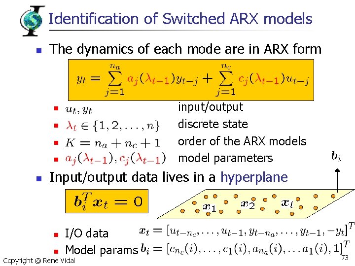
Identification of Switched ARX models n The dynamics of each mode are in ARX form input/output discrete state order of the ARX models model parameters n n n Input/output data lives in a hyperplane n I/O data Model params n Copyright @ Rene Vidal 73

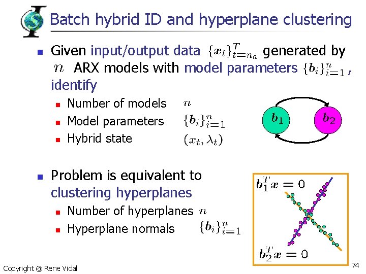
Batch hybrid ID and hyperplane clustering n Given input/output data generated by ARX models with model parameters , identify n n Number of models Model parameters Hybrid state Problem is equivalent to clustering hyperplanes n n Number of hyperplanes Hyperplane normals Copyright @ Rene Vidal 74

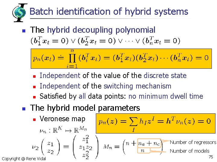
Batch identification of hybrid systems n The hybrid decoupling polynomial n n Independent of the value of the discrete state Independent of the switching mechanism Satisfied by all data points: no minimum dwell time The hybrid model parameters n Veronese map Number of regressors Number of models Copyright @ Rene Vidal 75

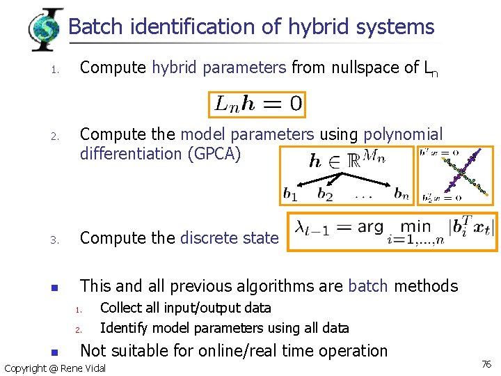
Batch identification of hybrid systems 1. 2. Compute hybrid parameters from nullspace of Ln Compute the model parameters using polynomial differentiation (GPCA) 3. Compute the discrete state n This and all previous algorithms are batch methods 1. 2. n Collect all input/output data Identify model parameters using all data Not suitable for online/real time operation Copyright @ Rene Vidal 76

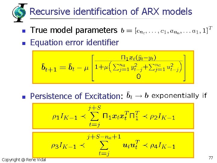
Recursive identification of ARX models n True model parameters Equation error identifier n Persistence of Excitation: n Copyright @ Rene Vidal 77

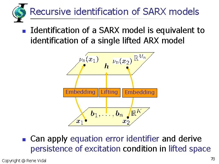
Recursive identification of SARX models n Identification of a SARX model is equivalent to identification of a single lifted ARX model Embedding n Lifting Embedding Can apply equation error identifier and derive persistence of excitation condition in lifted space Copyright @ Rene Vidal 78

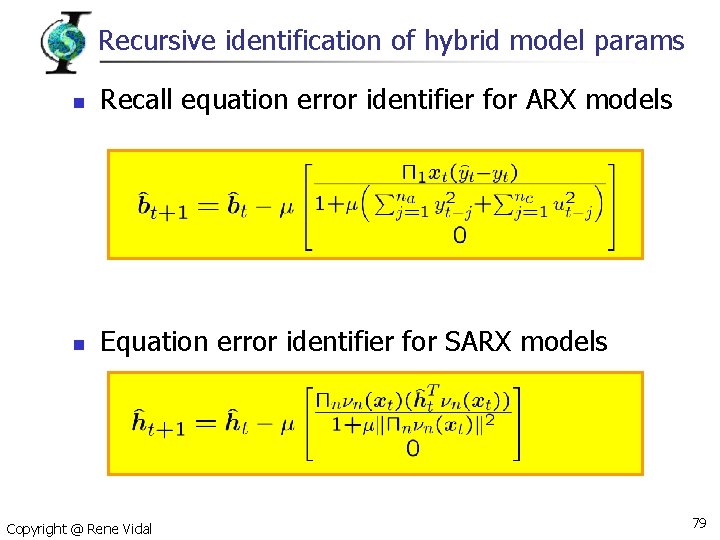
Recursive identification of hybrid model params n Recall equation error identifier for ARX models n Equation error identifier for SARX models Copyright @ Rene Vidal 79

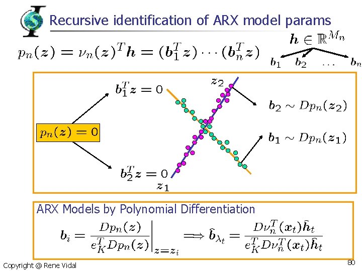
Recursive identification of ARX model params ARX Models by Polynomial Differentiation Copyright @ Rene Vidal 80

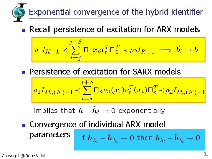
Exponential convergence of the hybrid identifier n Recall persistence of excitation for ARX models n Persistence of excitation for SARX models n Convergence of individual ARX model parameters Copyright @ Rene Vidal 81

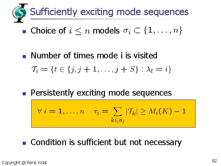
Sufficiently exciting mode sequences n Choice of n Number of times mode i is visited n Persistently exciting mode sequences n Condition is sufficient but not necessary Copyright @ Rene Vidal models 82

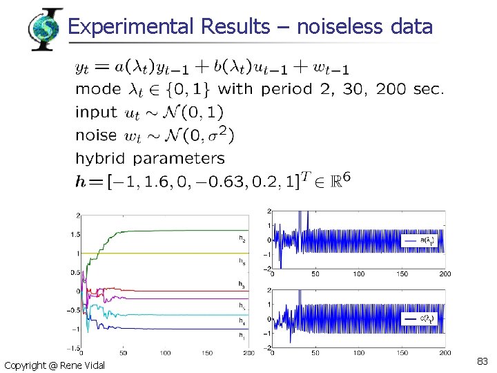
Experimental Results – noiseless data Copyright @ Rene Vidal 83

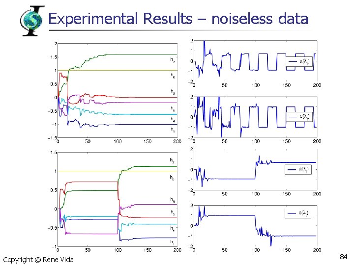
Experimental Results – noiseless data Copyright @ Rene Vidal 84

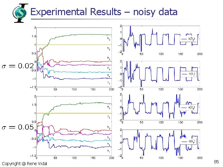
Experimental Results – noisy data Copyright @ Rene Vidal 85

Conclusions and open issues n Contributions n n n A recursive identification algorithm for hybrid ARX models of equal and known orders A persistence of excitation condition on the input/output data that guarantees exponential convergence Open issues n n n Persistence of excitation condition on the mode and input sequences only Recursive algorithm for identifying the parameters of SARX models of unknown and different orders Extend the model to multivariate SARX models Copyright @ Rene Vidal 86

References Copyright @ Rene Vidal 87

Thanks to collaborators and Ph. D students n University of Illinois n n n Yi Ma Kun Huang Johns Hopkins University n n n Jacopo Piazzi Alvina Goh Dheeraj Singaraju Avinash Ravishandran Copyright @ Rene Vidal Australian National University n n UCLA n n Richard Hartley Stefano Soatto UC Berkeley n Shankar Sastry 88