Linear Regression 1 What is a linear regression

Linear Regression 1

• • What is a linear regression How do we make a linear regression Assessing the model Demo in Python 2

What is linear regression? • Regression is an approach/method/algorithm used in finding the relationship between explanatory variables (or independent variables) and our variable of interest (or dependent variable). 3

What is linear regression? • Said another way, we are interested in finding out how much our variable of interest (Y), will increase (or decrease) with a change in each of our explanatory/indep. variables (X 1, X 2, …) 4

Examples • I work at Adobe. Work with lots of online retailers. A very common question is “How much is a visit worth (in terms of revenue)? ” – How is Revenue (Y) related to number of visits (X)? – Natural extension of this is how is revenue related to different types of visits (google search, direct type, email campaign, etc. )? 5

Examples • How can I estimate the value of a car? – Simple approach = value of car by the odometer – Advanced approach = for each make and model, how do the odometer reading change the value. 6

Examples • What are some factors that influence house prices and how much do they influence them? – Price (Y) related to: • • • Number of bedrooms (X 1) Number of bathrooms (X 2) Square footage (X 3) Lot size (X 4) Etc. 7

How do we create a linear regression? 8

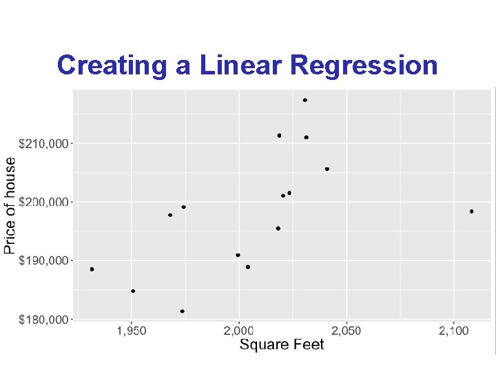
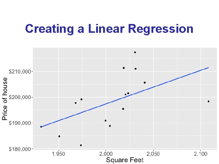
Creating a Linear Regression 9

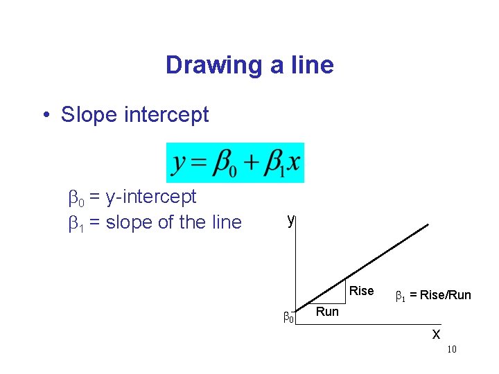
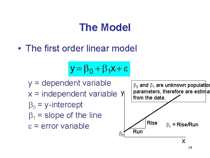
Drawing a line • Slope intercept b 0 = y-intercept b 1 = slope of the line y Rise b 0 b 1 = Rise/Run x 10

Introduction • We will examine the relationship between quantitative variables x and y via a mathematical equation. • The motivation for using the technique: – Forecast the value of a dependent variable (y) from the value of independent variables (x 1, x 2, …xk. ). – Analyze the specific relationships between the independent variables and the 11 dependent variable.

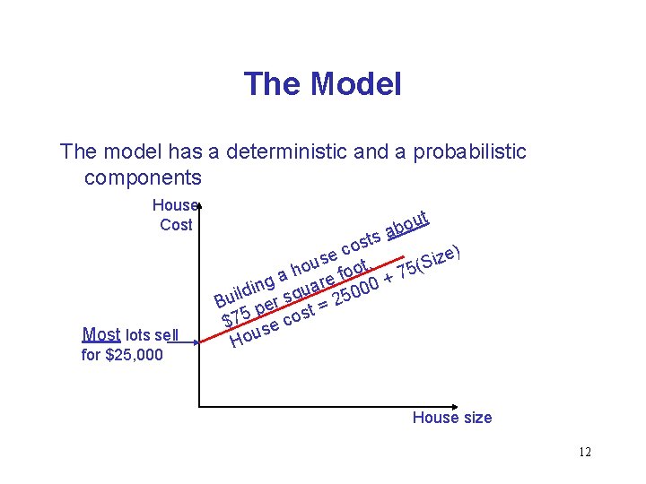
The Model The model has a deterministic and a probabilistic components House Cost Most lots sell for $25, 000 ut o b a s ost c ) e e z s i hou foot. + 75(S a g re 00 n a i u d l 0 Bui per sq t = 25 s $75 se co House size 12

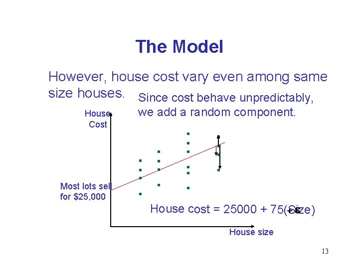
The Model However, house cost vary even among same size houses. Since cost behave unpredictably, House Cost Most lots sell for $25, 000 we add a random component. House cost = 25000 + 75(Size) +e House size 13

The Model • The first order linear model y = dependent variable x = independent variable y b 0 = y-intercept b 1 = slope of the line e = error variable b 0 and b 1 are unknown population parameters, therefore are estimat from the data. Rise b 1 = Rise/Run x 14

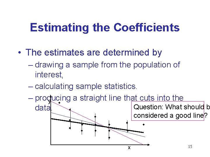
Estimating the Coefficients • The estimates are determined by – drawing a sample from the population of interest, – calculating sample statistics. – producing a straight line that cuts into the y w Question: What should b data. w w w considered a good line? w w w x 15

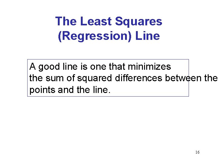
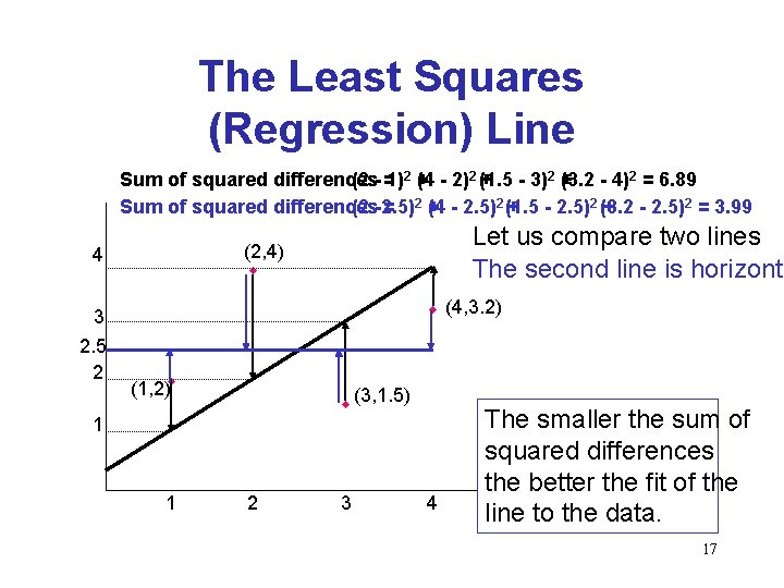
The Least Squares (Regression) Line A good line is one that minimizes the sum of squared differences between the points and the line. 16

The Least Squares (Regression) Line Sum of squared differences (2 - =1)2 + (4 - 2)2 (+1. 5 - 3)2 + (3. 2 - 4)2 = 6. 89 Sum of squared differences (2 -2. 5) = 2+ (4 - 2. 5)2 (+1. 5 - 2. 5)2 (3. 2 + - 2. 5)2 = 3. 99 3 2. 5 2 Let us compare two lines The second line is horizonta (2, 4) w 4 w (4, 3. 2) (1, 2)w w (3, 1. 5) 1 1 2 3 4 The smaller the sum of squared differences the better the fit of the line to the data. 17

Creating a Linear Regression 18

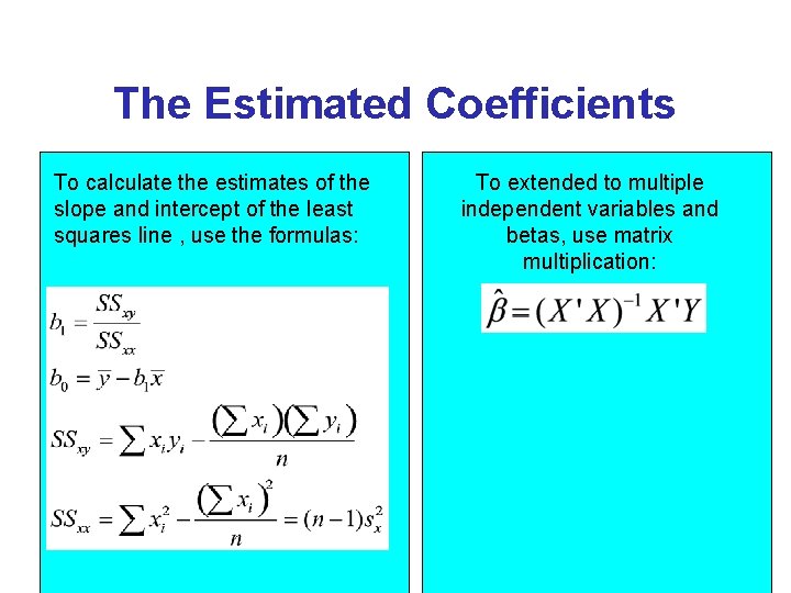
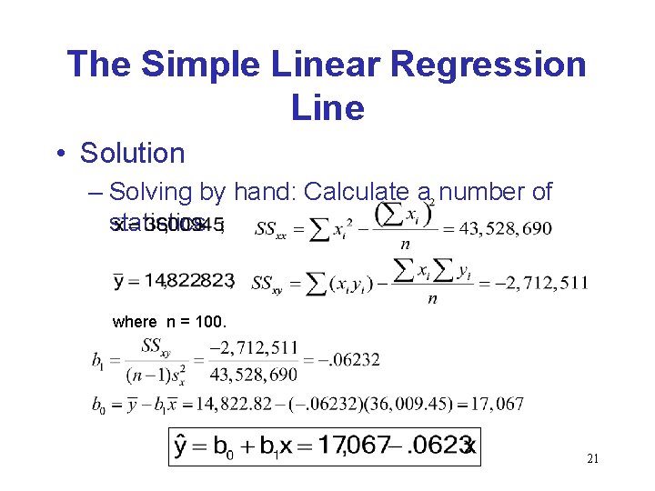
The Estimated Coefficients To calculate the estimates of the slope and intercept of the least squares line , use the formulas: To extended to multiple independent variables and betas, use matrix multiplication: 19

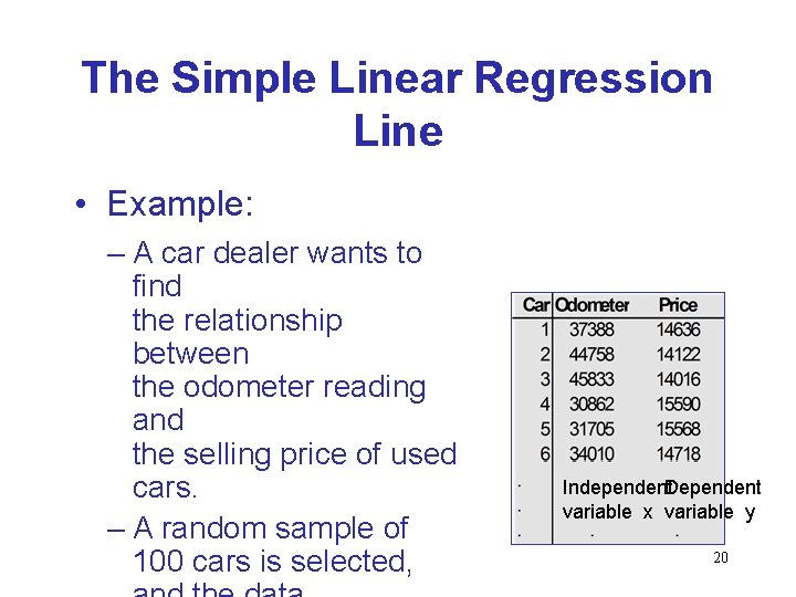
The Simple Linear Regression Line • Example: – A car dealer wants to find the relationship between the odometer reading and the selling price of used cars. – A random sample of 100 cars is selected, Independent. Dependent variable x variable y 20

The Simple Linear Regression Line • Solution – Solving by hand: Calculate a number of statistics where n = 100. 21

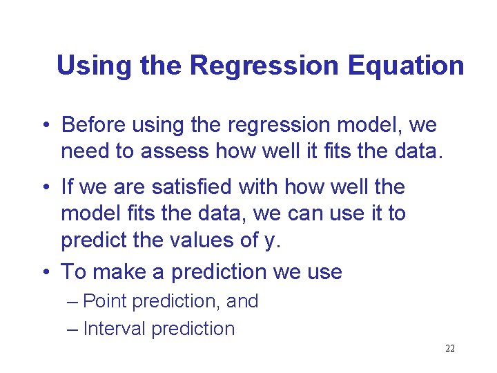
Using the Regression Equation • Before using the regression model, we need to assess how well it fits the data. • If we are satisfied with how well the model fits the data, we can use it to predict the values of y. • To make a prediction we use – Point prediction, and – Interval prediction 22

Assessing the model 23

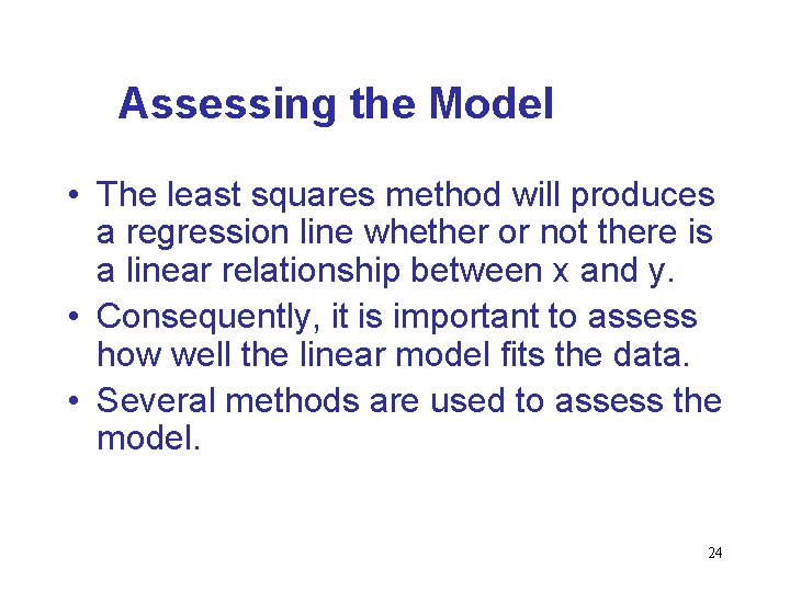
Assessing the Model • The least squares method will produces a regression line whether or not there is a linear relationship between x and y. • Consequently, it is important to assess how well the linear model fits the data. • Several methods are used to assess the model. 24

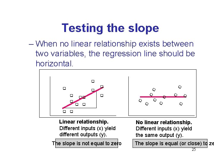
Testing the slope – When no linear relationship exists between two variables, the regression line should be horizontal. q q q qq q q q q Linear relationship. Different inputs (x) yield different outputs (y). The slope is not equal to zero No linear relationship. Different inputs (x) yield the same output (y). The slope is equal (or close) to ze 25

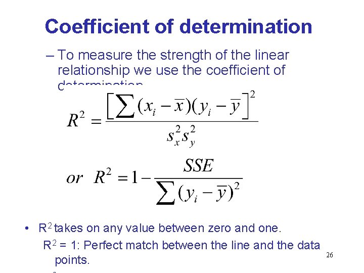
Coefficient of determination – To measure the strength of the linear relationship we use the coefficient of determination. • R 2 takes on any value between zero and one. R 2 = 1: Perfect match between the line and the data points. 26

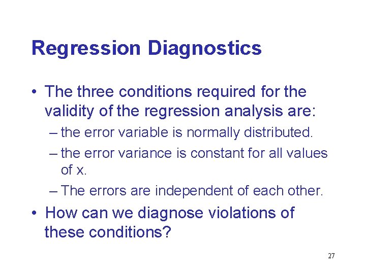
Regression Diagnostics • The three conditions required for the validity of the regression analysis are: – the error variable is normally distributed. – the error variance is constant for all values of x. – The errors are independent of each other. • How can we diagnose violations of these conditions? 27

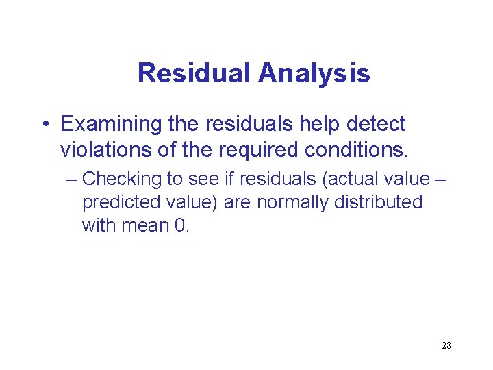
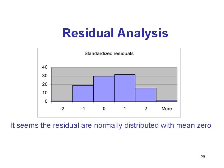
Residual Analysis • Examining the residuals help detect violations of the required conditions. – Checking to see if residuals (actual value – predicted value) are normally distributed with mean 0. 28

Residual Analysis It seems the residual are normally distributed with mean zero 29

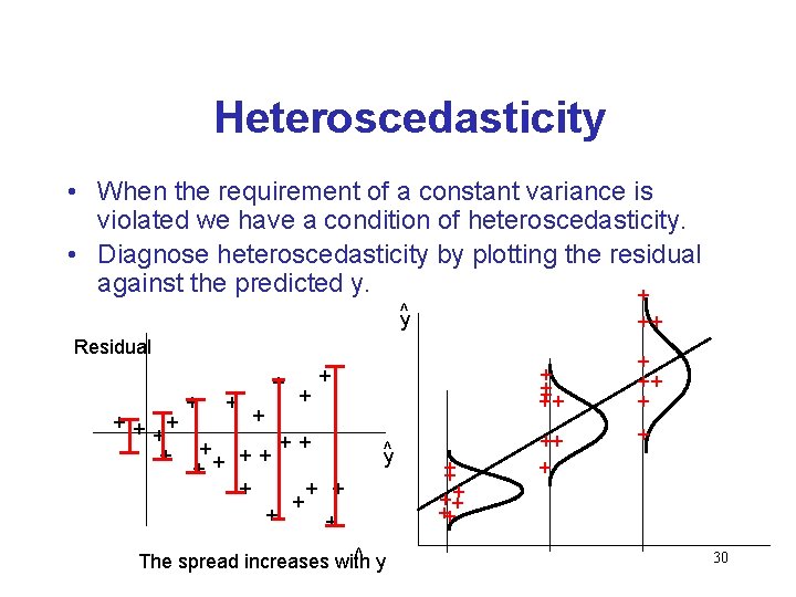
Heteroscedasticity • When the requirement of a constant variance is violated we have a condition of heteroscedasticity. • Diagnose heteroscedasticity by plotting the residual against the predicted y. + ^y ++ Residual + + + ++ + + + y^ ^ y The spread increases with + ++ ++ ++ + + 30

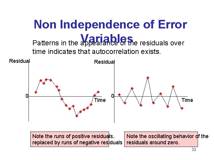
Non Independence of Error Variables – A time series is constituted if data were collected over time. – Examining the residuals over time, no pattern should be observed if the errors are independent. – When a pattern is detected, the errors are said to be autocorrelated. – Autocorrelation can be detected by graphing the residuals against time. 31

Non Independence of Error Variables Patterns in the appearance of the residuals over time indicates that autocorrelation exists. Residual + ++ + 0 + + ++ + 0 + Time + + Note the runs of positive residuals, Note the oscillating behavior of the replaced by runs of negative residuals around zero. 32

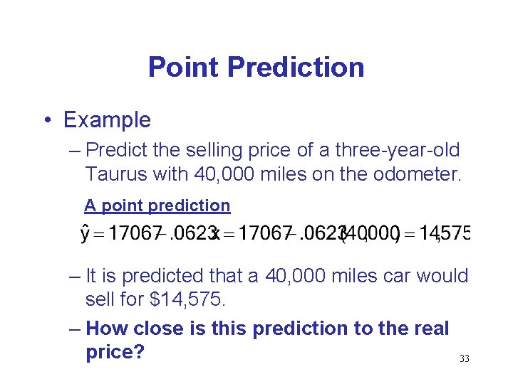
Point Prediction • Example – Predict the selling price of a three-year-old Taurus with 40, 000 miles on the odometer. A point prediction – It is predicted that a 40, 000 miles car would sell for $14, 575. – How close is this prediction to the real price? 33

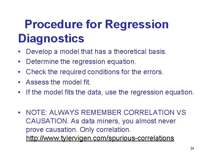
Procedure for Regression Diagnostics • • • Develop a model that has a theoretical basis. Determine the regression equation. Check the required conditions for the errors. Assess the model fit. If the model fits the data, use the regression equation. • NOTE: ALWAYS REMEMBER CORRELATION VS CAUSATION. As data miners, you almost never prove causation. Only correlation. http: //www. tylervigen. com/spurious-correlations 34