Inference for Linear Regression Conditions for Regression Inference

Inference for Linear Regression

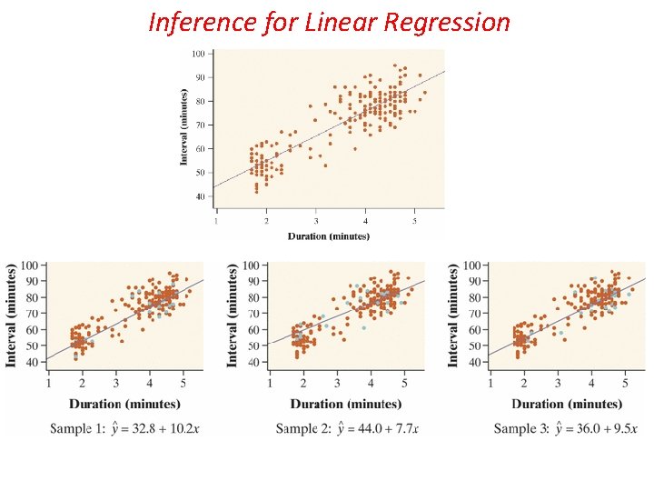
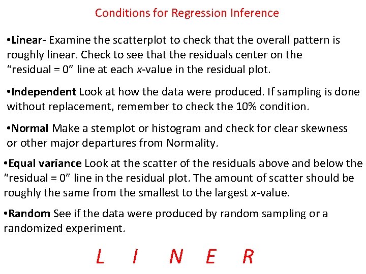
Conditions for Regression Inference • Linear- Examine the scatterplot to check that the overall pattern is roughly linear. Check to see that the residuals center on the “residual = 0” line at each x-value in the residual plot. • Independent Look at how the data were produced. If sampling is done without replacement, remember to check the 10% condition. • Normal Make a stemplot or histogram and check for clear skewness or other major departures from Normality. • Equal variance Look at the scatter of the residuals above and below the “residual = 0” line in the residual plot. The amount of scatter should be roughly the same from the smallest to the largest x-value. • Random See if the data were produced by random sampling or a randomized experiment. L I N E R

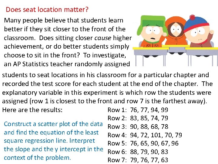
Does seat location matter? Many people believe that students learn better if they sit closer to the front of the classroom. Does sitting closer cause higher achievement, or do better students simply choose to sit in the front? To investigate, an AP Statistics teacher randomly assigned students to seat locations in his classroom for a particular chapter and recorded the test score for each student at the end of the chapter. The explanatory variable in this experiment is which row the students were assigned (row 1 is closest to the front and row 7 is the farthest away). Row 1: 76, 77, 94, 99 Here are the results: Row 2: 83, 85, 74, 79 Construct a scatter plot of the data Row 3: 90, 88, 68, 78 and find the equation of the least Row 4: 94, 72, 101, 70, 79 square regression line. Interpret Row 5: 76, 65, 90, 67, 96 the slope and the y intercept in the Row 6: 88, 79, 90, 83 context of the problem. Row 7: 79, 76, 77, 63

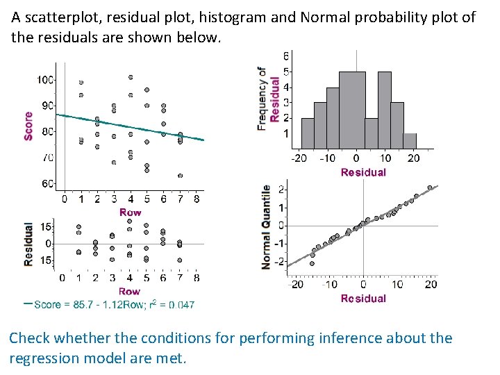
A scatterplot, residual plot, histogram and Normal probability plot of the residuals are shown below. Check whether the conditions for performing inference about the regression model are met.

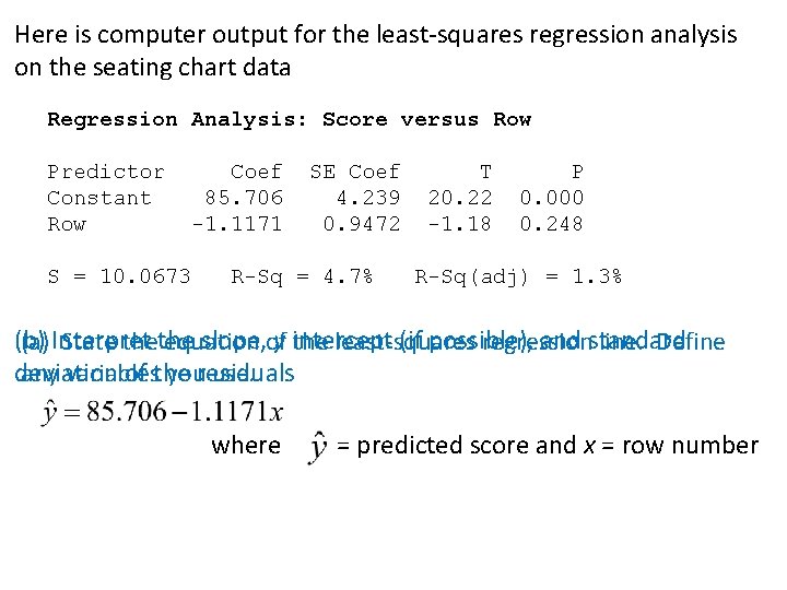
Here is computer output for the least-squares regression analysis on the seating chart data Regression Analysis: Score versus Row Predictor Coef SE Coef T P Constant 85. 706 4. 239 20. 22 0. 000 Row -1. 1171 0. 9472 -1. 18 0. 248 S = 10. 0673 R-Sq = 4. 7% R-Sq(adj) = 1. 3% (b) Interpret the slope, y intercept (if possible), and standard (a) State the equation of the least-squares regression line. Define any variables you use. deviation of the residuals where = predicted score and x = row number

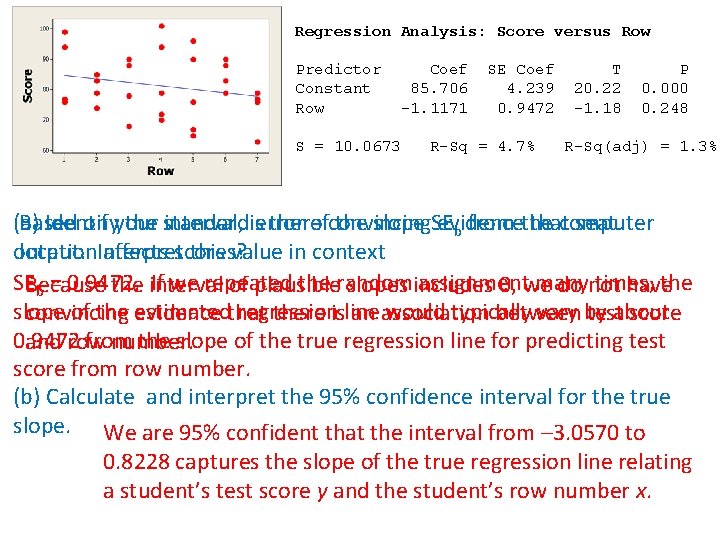
Regression Analysis: Score versus Row Predictor Coef SE Coef T P Constant 85. 706 4. 239 20. 22 0. 000 Row -1. 1171 0. 9472 -1. 18 0. 248 S = 10. 0673 R-Sq = 4. 7% R-Sq(adj) = 1. 3% (a) Identify the standard error of the slope SE Based on your interval, is there convincing evidence that seat b from the computer output. Interpret this value in context location affects scores? SEBecause the interval of plausible slopes includes 0, we do not have b = 0. 9472. If we repeated the random assignment many times, the slope of the estimated regression line would typically vary by about convincing evidence that there is an association between test score 0. 9472 from the slope of the true regression line for predicting test and row number. score from row number. (b) Calculate and interpret the 95% confidence interval for the true slope. We are 95% confident that the interval from – 3. 0570 to 0. 8228 captures the slope of the true regression line relating a student’s test score y and the student’s row number x.

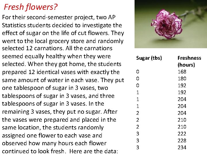
Fresh flowers? For their second-semester project, two AP Statistics students decided to investigate the effect of sugar on the life of cut flowers. They went to the local grocery store and randomly selected 12 carnations. All the carnations seemed equally healthy when they were selected. When they got home, the students prepared 12 identical vases with exactly the same amount of water in each vase. They put one tablespoon of sugar in 3 vases, two tablespoons of sugar in 3 vases, and three tablespoons of sugar in 3 vases. In the remaining 3 vases, they put no sugar. After the vases were prepared and placed in the same location, the students randomly assigned one flower to each vase and observed how many hours each flower continued to look fresh. Here are the data: Sugar (tbs) 0 0 0 1 1 1 2 2 2 3 3 3 Freshness (hours) 168 180 192 204 204 210 222 228 234

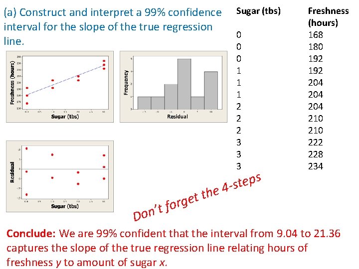
(a) Construct and interpret a 99% confidence interval for the slope of the true regression line. Sugar (tbs) 0 0 0 1 1 1 2 2 2 3 3 3 s p e t s e 4 - Freshness (hours) 168 180 192 204 204 210 222 228 234 h t t e org f t ’ n Do Conclude: We are 99% confident that the interval from 9. 04 to 21. 36 captures the slope of the true regression line relating hours of freshness y to amount of sugar x.

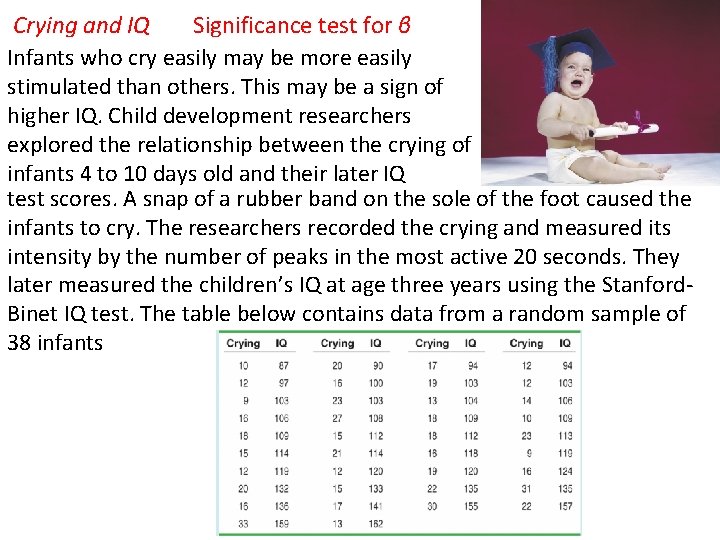
Crying and IQ Significance test for β Infants who cry easily may be more easily stimulated than others. This may be a sign of higher IQ. Child development researchers explored the relationship between the crying of infants 4 to 10 days old and their later IQ test scores. A snap of a rubber band on the sole of the foot caused the infants to cry. The researchers recorded the crying and measured its intensity by the number of peaks in the most active 20 seconds. They later measured the children’s IQ at age three years using the Stanford. Binet IQ test. The table below contains data from a random sample of 38 infants

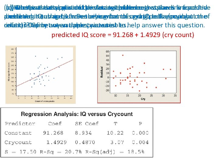
(b) What is the equation of the least-squares regression line for (a) Here is a scatterplot of the data with the least-squares line added (d) Do these data provide convincing evidence that there is a positive (c) Interpret the slope and y intercept of the regression line in and the minitab output. Describe what this graph tells you about the predicting IQ at age 3 from the number of crying peaks (crying linear relationship between crying counts and IQ in the population of context. relationship between these two variables. count)? Define any variables you use. infants? Carry out an appropriate test to help answer this question. predicted IQ score = 91. 268 + 1. 4929 (cry count)

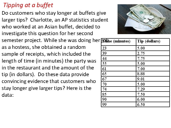
Tipping at a buffet Do customers who stay longer at buffets give larger tips? Charlotte, an AP statistics student who worked at an Asian buffet, decided to investigate this question for her second semester project. While she was doing her job Time (minutes) as a hostess, she obtained a random 23 39 sample of receipts, which included the length of time (in minutes) the party was 44 55 in the restaurant and the amount of the 61 65 tip (in dollars). Do these data provide convincing evidence that customers who 67 70 stay longer give larger tips? Here is the 74 85 data: 90 99 Tip (dollars) 5. 00 2. 75 7. 75 5. 00 7. 00 8. 88 9. 01 5. 00 7. 29 7. 50 6. 00 6. 50

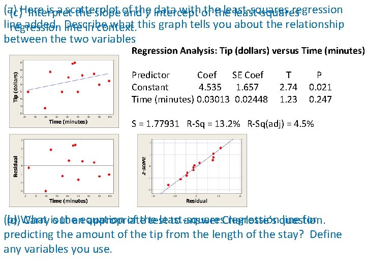
(a) Here is a scatterplot of the data with the least-squares regression (c) Interpret the slope and y intercept of the least-squares line added. Describe what this graph tells you about the relationship regression line in context. between the two variables Regression Analysis: Tip (dollars) versus Time (minutes) Predictor Coef SE Coef T P Constant 4. 535 1. 657 2. 74 0. 021 Time (minutes) 0. 03013 0. 02448 1. 23 0. 247 S = 1. 77931 R-Sq = 13. 2% R-Sq(adj) = 4. 5% (b) What is the equation of the least-squares regression line for (d) Carry out an appropriate test to answer Charlotte’s question. predicting the amount of the tip from the length of the stay? Define any variables you use.

Exercises on page 759, #5 -19 odds