Count Models Sociology 229 Advanced Regression Copyright 2010

Count Models Sociology 229: Advanced Regression Copyright © 2010 by Evan Schofer Do not copy or distribute without permission

Announcements • Assignment #1 Due • Assignment #2 handed out • Due in 1 week • Agenda: • Basic count models • Intro to EHA (if time allows)

Count Variables • Many dependent variables are counts: Nonnegative integers • • # Crimes a person has committed in lifetime # Children living in a household # new companies founded in a year (in an industry) # of social protests per month in a city – Can you think of others?

Count Variables • Count variables can be modeled with OLS regression… but: – 1. Linear models can yield negative predicted values… whereas counts are never negative • Similar to the problem of the Linear Probability Model – 2. Count variables are often highly skewed • Ex: # crimes committed this year… most people are zero or very low; a few people are very high • Extreme skew violates the normality assumption of OLS regression.

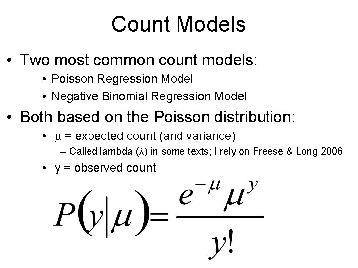
Count Models • Two most common count models: • Poisson Regression Model • Negative Binomial Regression Model • Both based on the Poisson distribution: • m = expected count (and variance) – Called lambda (l) in some texts; I rely on Freese & Long 2006 • y = observed count

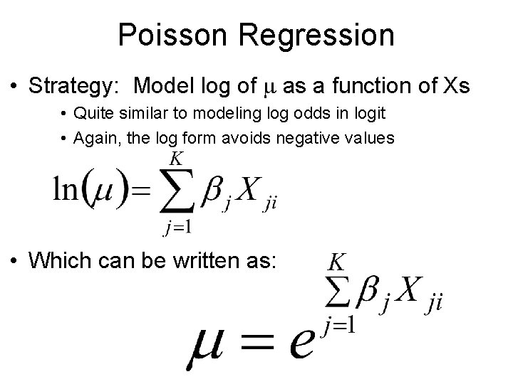
Poisson Regression • Strategy: Model log of m as a function of Xs • Quite similar to modeling log odds in logit • Again, the log form avoids negative values • Which can be written as:

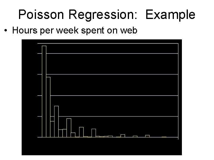
Poisson Regression: Example • Hours per week spent on web

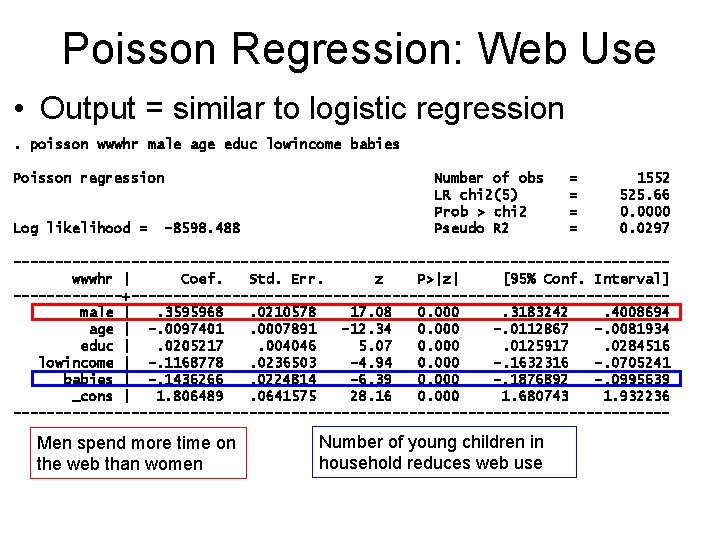
Poisson Regression: Web Use • Output = similar to logistic regression. poisson wwwhr male age educ lowincome babies Poisson regression Log likelihood = -8598. 488 Number of obs LR chi 2(5) Prob > chi 2 Pseudo R 2 = = 1552 525. 66 0. 0000 0. 0297 ---------------------------------------wwwhr | Coef. Std. Err. z P>|z| [95% Conf. Interval] -------+--------------------------------male |. 3595968. 0210578 17. 08 0. 000. 3183242. 4008694 age | -. 0097401. 0007891 -12. 34 0. 000 -. 0112867 -. 0081934 educ |. 0205217. 004046 5. 07 0. 000. 0125917. 0284516 lowincome | -. 1168778. 0236503 -4. 94 0. 000 -. 1632316 -. 0705241 babies | -. 1436266. 0224814 -6. 39 0. 000 -. 1876892 -. 0995639 _cons | 1. 806489. 0641575 28. 16 0. 000 1. 680743 1. 932236 --------------------------------------- Men spend more time on the web than women Number of young children in household reduces web use

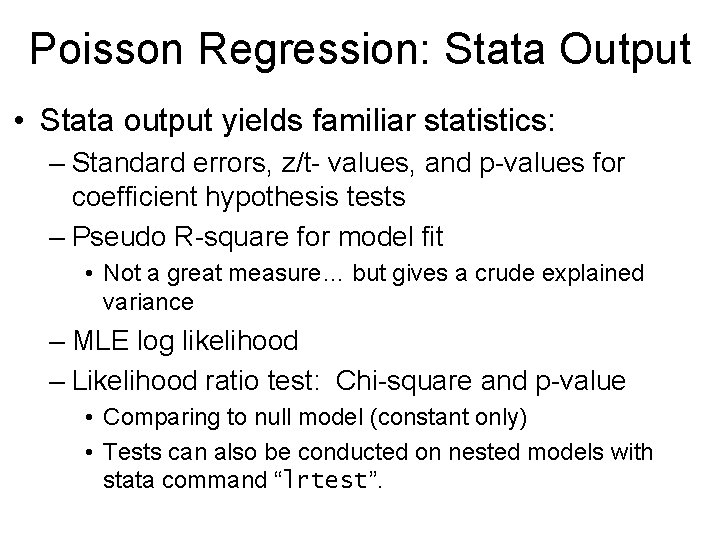
Poisson Regression: Stata Output • Stata output yields familiar statistics: – Standard errors, z/t- values, and p-values for coefficient hypothesis tests – Pseudo R-square for model fit • Not a great measure… but gives a crude explained variance – MLE log likelihood – Likelihood ratio test: Chi-square and p-value • Comparing to null model (constant only) • Tests can also be conducted on nested models with stata command “lrtest”.

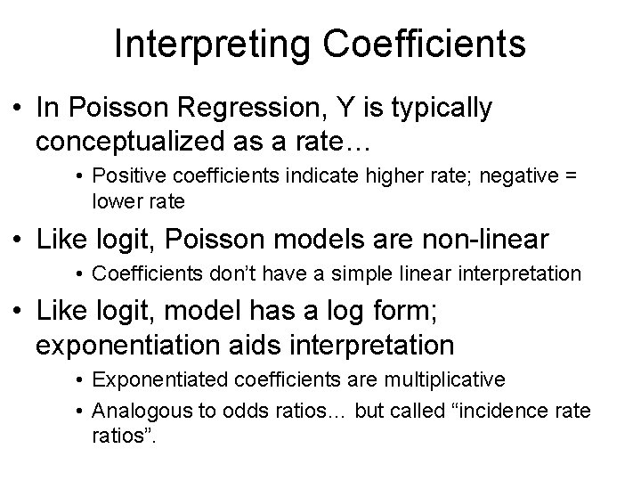
Interpreting Coefficients • In Poisson Regression, Y is typically conceptualized as a rate… • Positive coefficients indicate higher rate; negative = lower rate • Like logit, Poisson models are non-linear • Coefficients don’t have a simple linear interpretation • Like logit, model has a log form; exponentiation aids interpretation • Exponentiated coefficients are multiplicative • Analogous to odds ratios… but called “incidence ratios”.

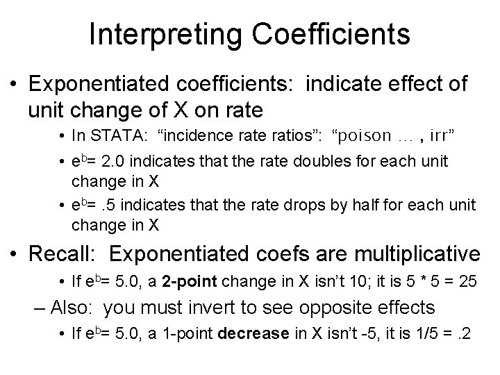
Interpreting Coefficients • Exponentiated coefficients: indicate effect of unit change of X on rate • In STATA: “incidence ratios”: “poison … , irr” • eb= 2. 0 indicates that the rate doubles for each unit change in X • eb=. 5 indicates that the rate drops by half for each unit change in X • Recall: Exponentiated coefs are multiplicative • If eb= 5. 0, a 2 -point change in X isn’t 10; it is 5 * 5 = 25 – Also: you must invert to see opposite effects • If eb= 5. 0, a 1 -point decrease in X isn’t -5, it is 1/5 =. 2

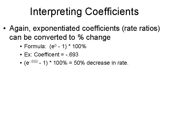
Interpreting Coefficients • Again, exponentiated coefficients (rate ratios) can be converted to % change • Formula: (eb - 1) * 100% • Ex: Coefficent = -. 693 • (e-. 693 - 1) * 100% = 50% decrease in rate.

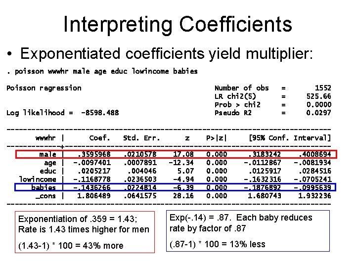
Interpreting Coefficients • Exponentiated coefficients yield multiplier: . poisson wwwhr male age educ lowincome babies Poisson regression Log likelihood = -8598. 488 Number of obs LR chi 2(5) Prob > chi 2 Pseudo R 2 = = 1552 525. 66 0. 0000 0. 0297 ---------------------------------------wwwhr | Coef. Std. Err. z P>|z| [95% Conf. Interval] -------+--------------------------------male |. 3595968. 0210578 17. 08 0. 000. 3183242. 4008694 age | -. 0097401. 0007891 -12. 34 0. 000 -. 0112867 -. 0081934 educ |. 0205217. 004046 5. 07 0. 000. 0125917. 0284516 lowincome | -. 1168778. 0236503 -4. 94 0. 000 -. 1632316 -. 0705241 babies | -. 1436266. 0224814 -6. 39 0. 000 -. 1876892 -. 0995639 _cons | 1. 806489. 0641575 28. 16 0. 000 1. 680743 1. 932236 --------------------------------------- Exponentiation of. 359 = 1. 43; Rate is 1. 43 times higher for men Exp(-. 14) =. 87. Each baby reduces rate by factor of. 87 (1. 43 -1) * 100 = 43% more (. 87 -1) * 100 = 13% less

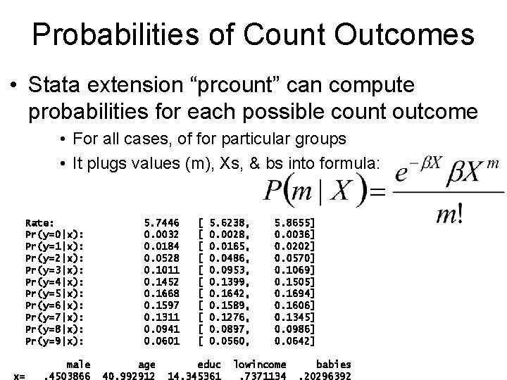
Probabilities of Count Outcomes • Stata extension “prcount” can compute probabilities for each possible count outcome • For all cases, of for particular groups • It plugs values (m), Xs, & bs into formula: Rate: Pr(y=0|x): Pr(y=1|x): Pr(y=2|x): Pr(y=3|x): Pr(y=4|x): Pr(y=5|x): Pr(y=6|x): Pr(y=7|x): Pr(y=8|x): Pr(y=9|x): x= male. 4503866 5. 7446 0. 0032 0. 0184 0. 0528 0. 1011 0. 1452 0. 1668 0. 1597 0. 1311 0. 0941 0. 0601 age 40. 992912 [ [ [ 5. 6238, 0. 0028, 0. 0165, 0. 0486, 0. 0953, 0. 1399, 0. 1642, 0. 1589, 0. 1276, 0. 0897, 0. 0560, educ 14. 345361 5. 8655] 0. 0036] 0. 0202] 0. 0570] 0. 1069] 0. 1505] 0. 1694] 0. 1606] 0. 1345] 0. 0986] 0. 0642] lowincome. 7371134 babies. 20296392

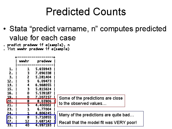
Predicted Counts • Stata “predict varname, n” computes predicted value for each case. predict predwww if e(sample), n. list wwwhr predwww if e(sample) 1. 2. 3. 12. 13. 15. 16. 19. 20. 21. 23. 24. 25. 27. 33. +---------+ | wwwhr predwww | |---------| | 1 5. 659943 | | 3 7. 090338 | | 2 5. 281404 | | 5 6. 09473 | | 4 6. 968055 | | 3 5. 815624 | | 0 5. 539187 | | 0 7. 207257 | | 8 8. 03906 | | 5 4. 400002 | | 1 6. 77004 | | 1 4. 806245 | | 8 5. 710855 | | 12 3. 687142 | | 40 4. 997193 | Some of the predictions are close to the observed values… Many of the predictions are quite bad… Recall that the model fit was VERY poor!

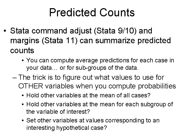
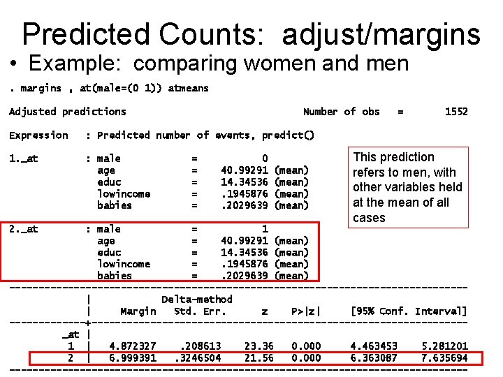
Predicted Counts • Stata command adjust (Stata 9/10) and margins (Stata 11) can summarize predicted counts • You can compute average predictions for each case in your data… or for sub-groups of the data. – The trick is to figure out what values to use for OTHER variables when you compute probabilities • Hold other variables at the mean of all cases? • Hold other variables at the mean for each subgroup of the variable of interest? • Set other variables at values corresponding to an interesting hypothetical case?

Predicted Counts: adjust/margins • Example: comparing women and men. margins , at(male=(0 1)) atmeans Adjusted predictions Number of obs Expression : Predicted number of events, predict() 1. _at : male age educ lowincome babies 2. _at = = = 0 40. 99291 14. 34536. 1945876. 2029639 (mean) = 1552 This prediction refers to men, with other variables held at the mean of all cases : male = 1 age = 40. 99291 (mean) educ = 14. 34536 (mean) lowincome =. 1945876 (mean) babies =. 2029639 (mean) ---------------------------------------| Delta-method | Margin Std. Err. z P>|z| [95% Conf. Interval] -------+--------------------------------_at | 1 | 4. 872327. 208613 23. 36 0. 000 4. 463453 5. 281201 2 | 6. 999391. 3246504 21. 56 0. 000 6. 363087 7. 635694 ---------------------------------------

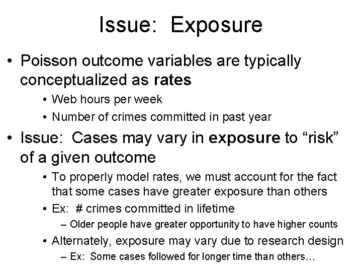
Issue: Exposure • Poisson outcome variables are typically conceptualized as rates • Web hours per week • Number of crimes committed in past year • Issue: Cases may vary in exposure to “risk” of a given outcome • To properly model rates, we must account for the fact that some cases have greater exposure than others • Ex: # crimes committed in lifetime – Older people have greater opportunity to have higher counts • Alternately, exposure may vary due to research design – Ex: Some cases followed for longer time than others…

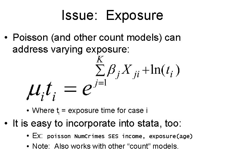
Issue: Exposure • Poisson (and other count models) can address varying exposure: • Where ti = exposure time for case i • It is easy to incorporate into stata, too: • Ex: poisson Num. Crimes SES income, exposure(age) • Note: Also works with other “count” models.

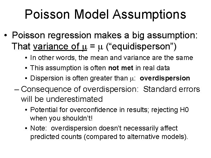
Poisson Model Assumptions • Poisson regression makes a big assumption: That variance of m = m (“equidisperson”) • In other words, the mean and variance are the same • This assumption is often not met in real data • Dispersion is often greater than m: overdispersion – Consequence of overdispersion: Standard errors will be underestimated • Potential for overconfidence in results; rejecting H 0 when you shouldn’t! • Note: overdispersion doesn’t necessarily affect predicted counts (compared to alternative models).

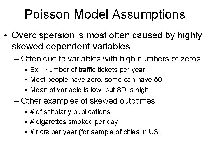
Poisson Model Assumptions • Overdispersion is most often caused by highly skewed dependent variables – Often due to variables with high numbers of zeros • Ex: Number of traffic tickets per year • Most people have zero, some can have 50! • Mean of variable is low, but SD is high – Other examples of skewed outcomes • # of scholarly publications • # cigarettes smoked per day • # riots per year (for sample of cities in US).

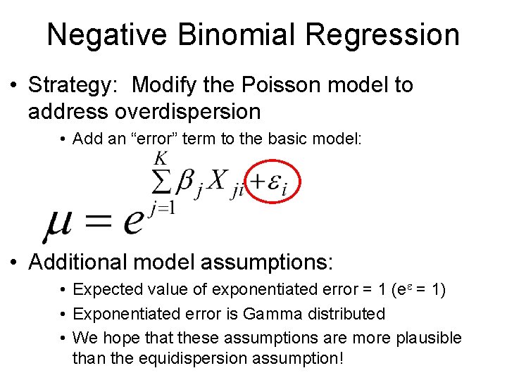
Negative Binomial Regression • Strategy: Modify the Poisson model to address overdispersion • Add an “error” term to the basic model: • Additional model assumptions: • Expected value of exponentiated error = 1 (ee = 1) • Exponentiated error is Gamma distributed • We hope that these assumptions are more plausible than the equidispersion assumption!

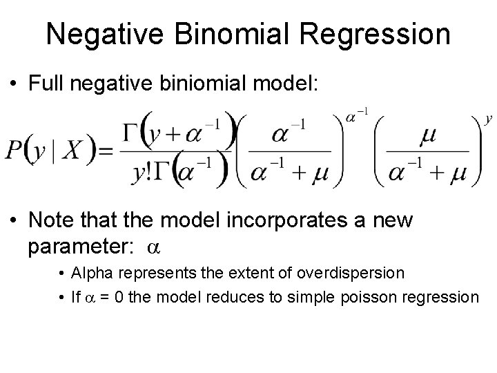
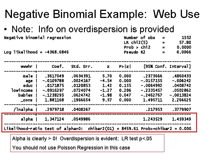
Negative Binomial Regression • Full negative biniomial model: • Note that the model incorporates a new parameter: a • Alpha represents the extent of overdispersion • If a = 0 the model reduces to simple poisson regression

Negative Binomial Regression • Question: Is alpha (a) = 0? • If so, we can use Poisson regression • If not, overdispersion is present; Poisson is inadequate • Strategy: conduct a statistical test of the hypothesis: H 0: a = 0; H 1: a > 0 • Stata provides this information when you run a negative binomial model: • Likelihood ratio test (G 2) for alpha • P-value <. 05 indicates that overdispersion is present; negative binomial is preferred • If P>. 05, just use Poisson regression – So you don’t have to make assumptions about gamma dist….

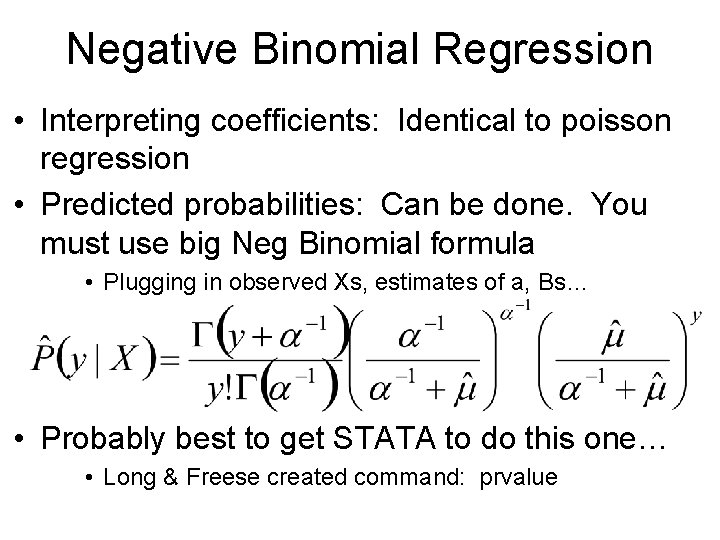
Negative Binomial Regression • Interpreting coefficients: Identical to poisson regression • Predicted probabilities: Can be done. You must use big Neg Binomial formula • Plugging in observed Xs, estimates of a, Bs… • Probably best to get STATA to do this one… • Long & Freese created command: prvalue

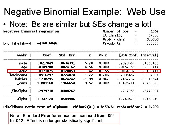
Negative Binomial Example: Web Use • Note: Bs are similar but SEs change a lot! Negative binomial regression Log likelihood = -4368. 6846 Number of obs LR chi 2(5) Prob > chi 2 Pseudo R 2 = = 1552 57. 80 0. 0000 0. 0066 ---------------------------------------wwwhr | Coef. Std. Err. z P>|z| [95% Conf. Interval] -------+--------------------------------male |. 3617049. 0634391 5. 70 0. 000. 2373666. 4860433 age | -. 0109788. 0024167 -4. 54 0. 000 -. 0157155 -. 006242 educ |. 0171875. 0120853 1. 42 0. 155 -. 0064992. 0408742 lowincome | -. 0916297. 0724074 -1. 27 0. 206 -. 2335457. 0502862 babies | -. 1238295. 0624742 -1. 98 0. 047 -. 2462767 -. 0013824 _cons | 1. 881168. 1966654 9. 57 0. 000 1. 495711 2. 266625 -------+--------------------------------/lnalpha |. 2979718. 0408267. 217953. 3779907 -------+--------------------------------alpha | 1. 347124. 0549986 1. 243529 1. 459349 ---------------------------------------Likelihood-ratio test of alpha=0: chibar 2(01) = 8459. 61 Prob>=chibar 2 = 0. 000 Note: Standard Error for education increased from. 004 to. 012! Effect is no longer statistically significant.

Negative Binomial Example: Web Use • Note: Info on overdispersion is provided Negative binomial regression Log likelihood = -4368. 6846 Number of obs LR chi 2(5) Prob > chi 2 Pseudo R 2 = = 1552 57. 80 0. 0000 0. 0066 ---------------------------------------wwwhr | Coef. Std. Err. z P>|z| [95% Conf. Interval] -------+--------------------------------male |. 3617049. 0634391 5. 70 0. 000. 2373666. 4860433 age | -. 0109788. 0024167 -4. 54 0. 000 -. 0157155 -. 006242 educ |. 0171875. 0120853 1. 42 0. 155 -. 0064992. 0408742 lowincome | -. 0916297. 0724074 -1. 27 0. 206 -. 2335457. 0502862 babies | -. 1238295. 0624742 -1. 98 0. 047 -. 2462767 -. 0013824 _cons | 1. 881168. 1966654 9. 57 0. 000 1. 495711 2. 266625 -------+--------------------------------/lnalpha |. 2979718. 0408267. 217953. 3779907 -------+--------------------------------alpha | 1. 347124. 0549986 1. 243529 1. 459349 ---------------------------------------Likelihood-ratio test of alpha=0: chibar 2(01) = 8459. 61 Prob>=chibar 2 = 0. 000 Alpha is clearly > 0! Overdispersion is evident; LR test p<. 05 You should not use Poisson Regression in this case

General Remarks • Poisson & Negative binomial models suffer all the same basic issues as “normal” regression • Model specification / omitted variable bias • Multicollinearity • Outliers/influential cases – Also, it uses Maximum Likelihood • N > 500 = fine; N < 100 can be worrisome – Results aren’t necessarily wrong if N<100; – But it is a possibility; and hard to know when problems crop up • Plus ~10 cases per independent variable.

General Remarks • It is often useful to try both Poisson and Negative Binomial models • The latter allows you to test for overdispersion • Use LRtest on alpha (a) to guide model choice – If you don’t suspect dispersion and alpha appears to be zero, use Poission Regression • It makes fewer assumptions – Such as gamma-distributed error.

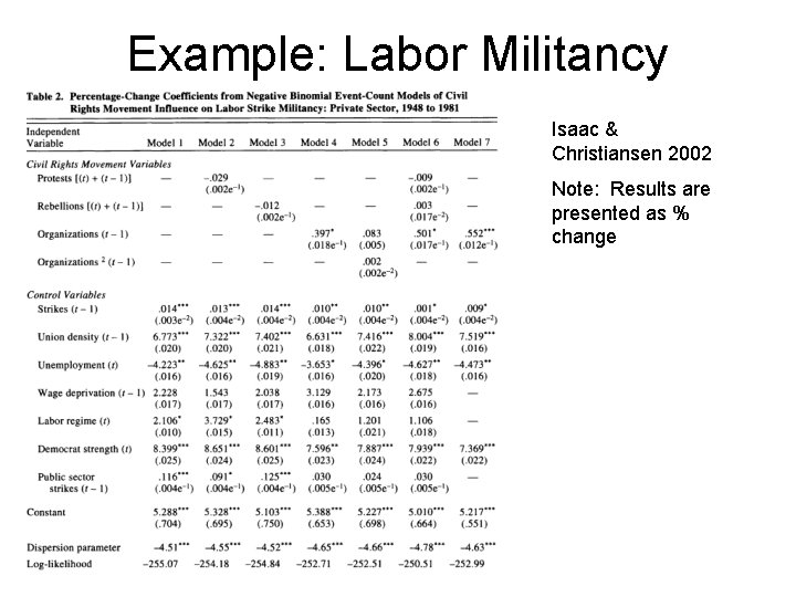
Example: Labor Militancy Isaac & Christiansen 2002 Note: Results are presented as % change

Zero-Inflated Poisson & NB Reg • If outcome variable has many zero values it tends to be highly skewed • Under those circumstances, NBREG works better than ordinary Poisson due to overdispersion – But, sometimes you have LOTS of zeros. Even nbreg isn’t sufficient • Model under-predicts zeros, doesn’t fit well – Examples: • # violent crimes committed by a person in a year • # of wars a country fights per year • # of foreign subsidiaries of firms.

Zero-Inflated Poisson & NB Reg • Logic of zero-inflated models: Assume two types of groups in your sample • Type A: Always zero – no probability of non-zero value • Type ~A: Non-zero chance of positive count value – Probability is variable, but not zero – 1. Use logit to model group membership – 2. Use poisson or nbreg to model counts for those in group ~A – 3. Compute probabilities based on those results.

Zero-Inflated Poisson & NB Reg • Example: Web usage at work • More skewed than overall web usage. Why? Many people don’t have computers at work! So, web usage is zero for many

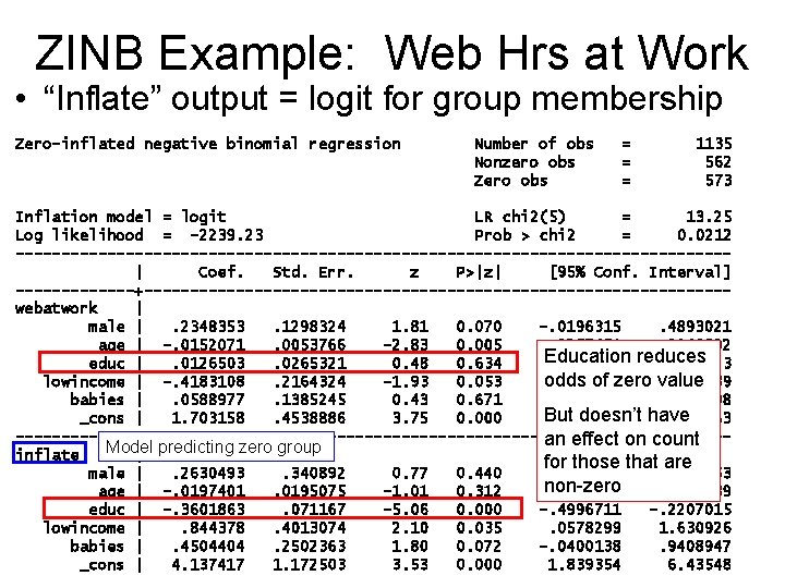
Zero-Inflated Poisson & NB Reg • Zero-inflated models in Stata • “zip” = Poisson, zinb = negative binomial • Commands accept two separate variable lists – Variables that affect counts • For those with non-zero counts • Modeled with Poisson or NB regression – Variables that predict membership in “zero” group • Modeled with logit – Ex: zinb webatwork male age educ lowincome babies, inflate(male age educ lowincome babies)

ZINB Example: Web Hrs at Work • “Inflate” output = logit for group membership Zero-inflated negative binomial regression Number of obs Nonzero obs Zero obs = = = 1135 562 573 Inflation model = logit LR chi 2(5) = 13. 25 Log likelihood = -2239. 23 Prob > chi 2 = 0. 0212 ---------------------------------------| Coef. Std. Err. z P>|z| [95% Conf. Interval] -------+--------------------------------webatwork | male |. 2348353. 1298324 1. 81 0. 070 -. 0196315. 4893021 age | -. 0152071. 0053766 -2. 83 0. 005 -. 0257451 -. 0046692 Education reduces educ |. 0126503. 0265321 0. 48 0. 634 -. 0393517. 0646523 odds of zero value lowincome | -. 4183108. 2164324 -1. 93 0. 053 -. 8425105. 0058889 babies |. 0588977. 1385245 0. 43 0. 671 -. 2126053. 3304008 But doesn’t have _cons | 1. 703158. 4538886 3. 75 0. 000. 8135524 2. 592763 -------+--------------------------------an effect on count Model inflate | predicting zero group for those that. 9311853 are male |. 2630493. 340892 0. 77 0. 440 -. 4050866 non-zero age | -. 0197401. 0195075 -1. 01 0. 312 -. 057974. 0184939 educ | -. 3601863. 071167 -5. 06 0. 000 -. 4996711 -. 2207015 lowincome |. 844378. 4013074 2. 10 0. 035. 0578299 1. 630926 babies |. 4504404. 2502363 1. 80 0. 072 -. 0400138. 9408947 _cons | 4. 137417 1. 172503 3. 53 0. 000 1. 839354 6. 43548

Zero-Inflated Poisson & NB Reg • Remarks – ZINB produces estimate of alpha • Helps choose between zip & zinb – Long and Freese (2006) have helpful tool to compare fit of count models: countfit • See textbook – Zero-inflated models seem very useful • Count variables often have many zeros • It is often reasonable to assume a “always zero” group – But, they are fairly new • Not many examples in the literature • Haven’t been widely scrutinized.

Zero-truncated Poisson & NB reg • Truncation – the absence of information about cases in some range of a variable • Example: Suppose we study income based on data from tax returns… – Cases with income below a certain value are not required to submit a tax return… so data is missing • Example: Data on # crimes committed, taken from legal records – Individuals with zero crimes are not evident in data • Example: An on-line survey of web use – Individuals with zero web use are not in data • Poisson & NB have been adapted to address truncated data: – Zero-truncated Poisson & Zero-trunciated NB reg.

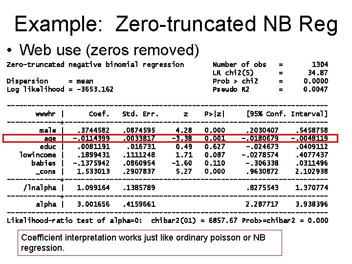
Example: Zero-truncated NB Reg • Web use (zeros removed) Zero-truncated negative binomial regression Dispersion = mean Log likelihood = -3653. 162 Number of obs LR chi 2(5) Prob > chi 2 Pseudo R 2 = = 1304 34. 87 0. 0000 0. 0047 ---------------------------------------wwwhr | Coef. Std. Err. z P>|z| [95% Conf. Interval] -------+--------------------------------male |. 3744582. 0874595 4. 28 0. 000. 2030407. 5458758 age | -. 0114399. 0033817 -3. 38 0. 001 -. 0180679 -. 0048119 educ |. 0081191. 016731 0. 49 0. 627 -. 024673. 0409112 lowincome |. 1899431. 1111248 1. 71 0. 087 -. 0278574. 4077437 babies | -. 1375942. 0860954 -1. 60 0. 110 -. 306338. 0311496 _cons | 1. 533013. 2907837 5. 27 0. 000. 9630872 2. 102938 -------+--------------------------------/lnalpha | 1. 099164. 1385789. 8275543 1. 370774 -------+--------------------------------alpha | 3. 001656. 4159661 2. 287717 3. 938396 ---------------------------------------Likelihood-ratio test of alpha=0: chibar 2(01) = 6857. 67 Prob>=chibar 2 = 0. 000 Coefficient interpretation works just like ordinary poisson or NB regression.

Empirical Example 2 • Example: Haynie, Dana L. 2001. “Delinquent Peers Revisited: Does Network Structure Matter? ” American Journal of Sociology, 106, 4: 1013 -1057.