Regression Models Introduction In regression models two types
- Slides: 8

Regression Models - Introduction • In regression models, two types of variables that are studied: Ø A dependent variable, Y, also called response variable. It is modeled as random. Ø An independent variable, X, also called predictor variable or explanatory variable. It is sometimes modeled as random and sometimes it has fixed value for each observation. • In regression models we are fitting a statistical model to data. • We generally use regression to be able to predict the value of one variable given the value of others. STA 302/1001 week 1 1

Simple Linear Regression - Introduction • Simple linear regression studies the relationship between a quantitative response variable Y, and a single explanatory variable X. • Idea of statistical model: Actual observed value of Y = … • Box (a well know statistician) claim: “All models are wrong, some are useful”. ‘Useful’ means that they describe the data well and can be used for predictions and inferences. • Recall: parameters are constants in a statistical model which we usually don’t know but will use data to estimate. STA 302/1001 week 1 2

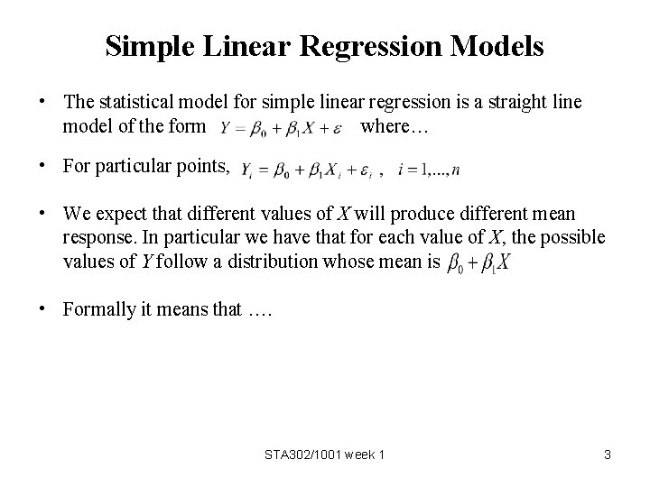
Simple Linear Regression Models • The statistical model for simple linear regression is a straight line model of the form where… • For particular points, • We expect that different values of X will produce different mean response. In particular we have that for each value of X, the possible values of Y follow a distribution whose mean is • Formally it means that …. STA 302/1001 week 1 3

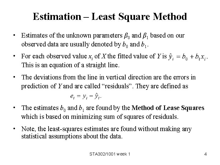
Estimation – Least Square Method • Estimates of the unknown parameters β 0 and β 1 based on our observed data are usually denoted by b 0 and b 1. • For each observed value xi of X the fitted value of Y is This is an equation of a straight line. • The deviations from the line in vertical direction are the errors in prediction of Y and are called “residuals”. They are defined as • The estimates b 0 and b 1 are found by the Method of Lease Squares which is based on minimizing sum of squares of residuals. • Note, the least-squares estimates are found without making any statistical assumptions about the data. STA 302/1001 week 1 4

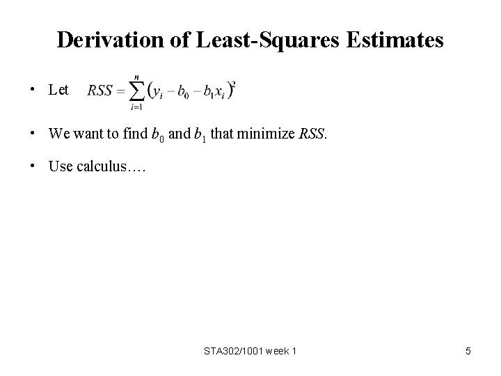
Derivation of Least-Squares Estimates • Let • We want to find b 0 and b 1 that minimize RSS. • Use calculus…. STA 302/1001 week 1 5

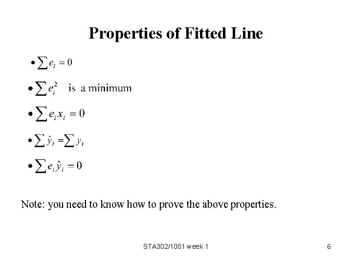
Properties of Fitted Line Note: you need to know how to prove the above properties. STA 302/1001 week 1 6

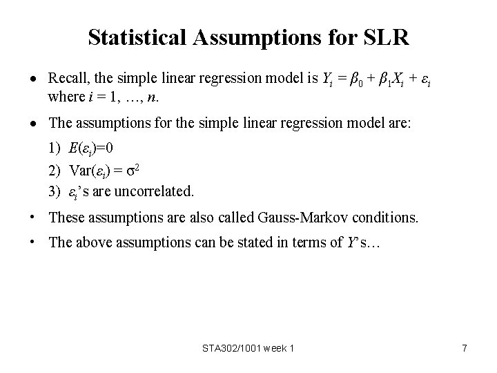
Statistical Assumptions for SLR Recall, the simple linear regression model is Yi = β 0 + β 1 Xi + εi where i = 1, …, n. The assumptions for the simple linear regression model are: 1) E(εi)=0 2) Var(εi) = σ2 3) εi’s are uncorrelated. • These assumptions are also called Gauss-Markov conditions. • The above assumptions can be stated in terms of Y’s… STA 302/1001 week 1 7

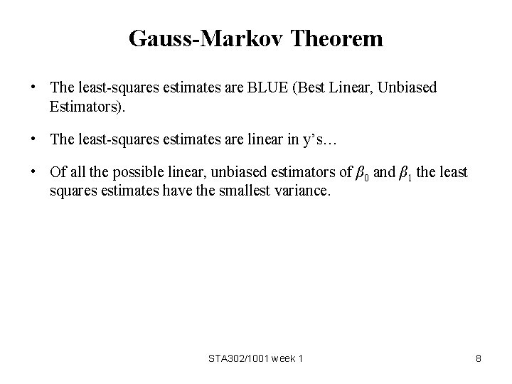
Gauss-Markov Theorem • The least-squares estimates are BLUE (Best Linear, Unbiased Estimators). • The least-squares estimates are linear in y’s… • Of all the possible linear, unbiased estimators of β 0 and β 1 the least squares estimates have the smallest variance. STA 302/1001 week 1 8