Generalized Linear Models All the regression models treated

Generalized Linear Models • All the regression models treated so far have common structure. This structure can be split up into two parts: ü The random part: ü The systematic part: • These two elements are the basic building blocks of generalized linear models.

The systematic part • Generalized linear model, systematic part: ü The covariates influence the distribution of response through the linear predictor: ü There is a link-function that links the expectation to the linear predictor:

The generalization from linear models to GLM • GLMs are a generalization of linear normal models in two directions:

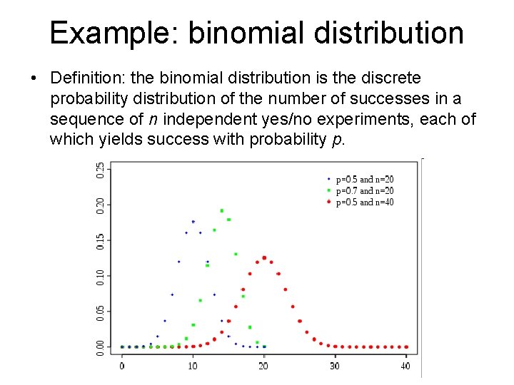
Example: binomial distribution • Definition: the binomial distribution is the discrete probability distribution of the number of successes in a sequence of n independent yes/no experiments, each of which yields success with probability p.

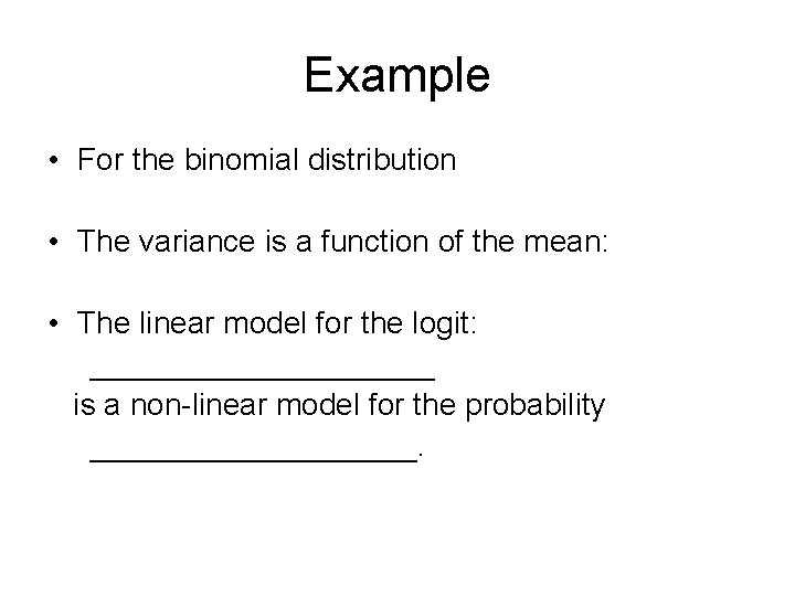
Example • For the binomial distribution • The variance is a function of the mean: • The linear model for the logit: __________ is a non-linear model for the probability __________.

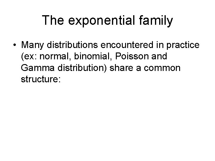
The exponential family • Many distributions encountered in practice (ex: normal, binomial, Poisson and Gamma distribution) share a common structure:

Example of the exponential family: Normal distribution

Example of the exponential family: Binomial

Example of the exponential family • The Poisson distribution: It is a discrete probability distribution that expresses the probability of a number of events occurring in a fixed period of time if these events occur with a known average rate and independently to the time. • Ex: ü The number of phone calls received by a telephone operator in a 10 -minute period. ü The number of typos per page made by a secretary.

Poisson distribution • The Poisson distribution belongs to the exponential family:

Mean and variance in the exponential family • It can be shown that the mean and variance in the exponential family is:

Mean and variance example: Poisson • For the Poisson model, mean and variance are: • To summarize, for any given distribution we obtain a specific form of b which in turn determines the variance function. • The converse is also true: • Hence specifying a distribution and a variance function is two sides of the same coin as long as we work with exponential families.

Various variance functions

The link function • The link function is a function which relates the mean to the linear predictor: • Various link functions have been illustrated so far:

Canonical link • For each distribution there is a specific link function which yields “nice” mathematical and numerical properties in connection with the estimation process. This link function is called the canonical link:

Specification of GLM • In practice, a GLM is specified by three steps: • In this connection it is important to be aware of the following: Most statistical packages will by default use the canonical link function unless another one is explicitly provided.

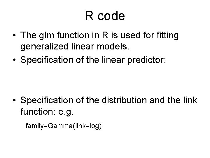
R code • The glm function in R is used for fitting generalized linear models. • Specification of the linear predictor: • Specification of the distribution and the link function: e. g. family=Gamma(link=log)

• Remember that the specification of a distribution yields a specific variance function. Not all possible combinations of a distribution and a link function are allowed in R.

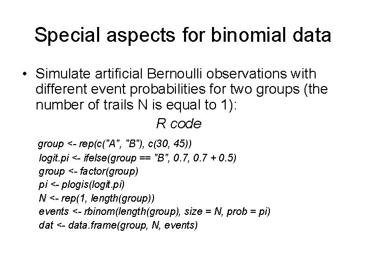
Special aspects for binomial data • Simulate artificial Bernoulli observations with different event probabilities for two groups (the number of trails N is equal to 1): R code group <- rep(c("A", "B"), c(30, 45)) logit. pi <- ifelse(group == "B", 0. 7 + 0. 5) group <- factor(group) pi <- plogis(logit. pi) N <- rep(1, length(group)) events <- rbinom(length(group), size = N, prob = pi) dat <- data. frame(group, N, events)

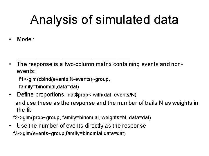
Analysis of simulated data • Model: __________________ • The response is a two-column matrix containing events and nonevents: f 1<-glm(cbind(events, N-events)~group, family=binomial, data=dat) • Define proportions: dat$prop<-with(dat, events/N) and use these as the response and the number of trails N as weights in the fit: f 2<-glm(prop~group, family=binomial, weights=N, data=dat) • Use the number of events directly as the response f 3<-glm(events~group, family=binomial, data=dat)

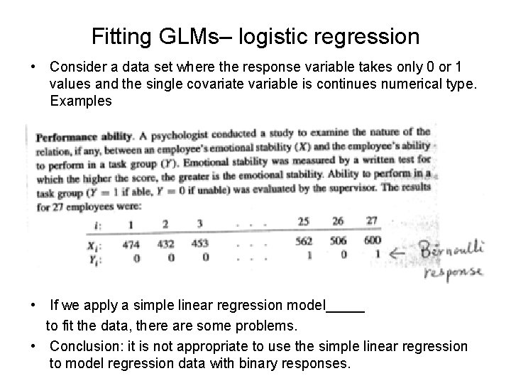
Fitting GLMs– logistic regression • Consider a data set where the response variable takes only 0 or 1 values and the single covariate variable is continues numerical type. Examples • If we apply a simple linear regression model_____ to fit the data, there are some problems. • Conclusion: it is not appropriate to use the simple linear regression to model regression data with binary responses.

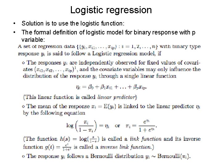
Logistic regression • Solution is to use the logistic function: • The formal definition of logistic model for binary response with p variable:

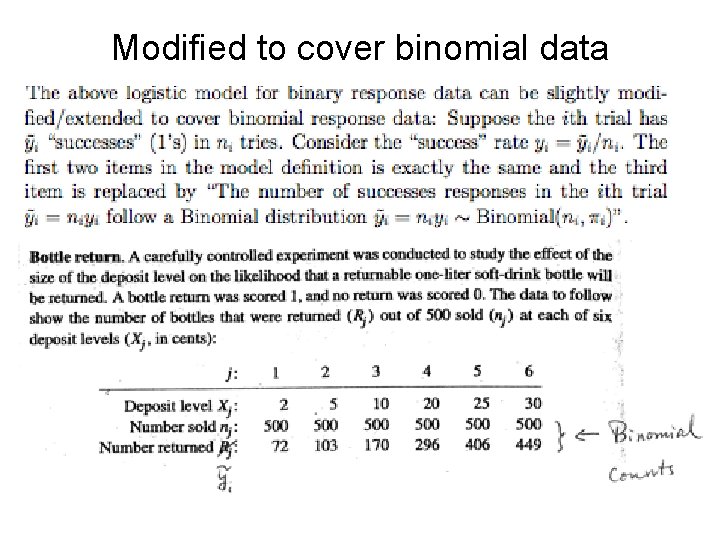
Logistic regression • How to interpret the model? • In logistic model, the odds of “success”: • The logistic model for binary data can be slightly modified

Modified to cover binomial data

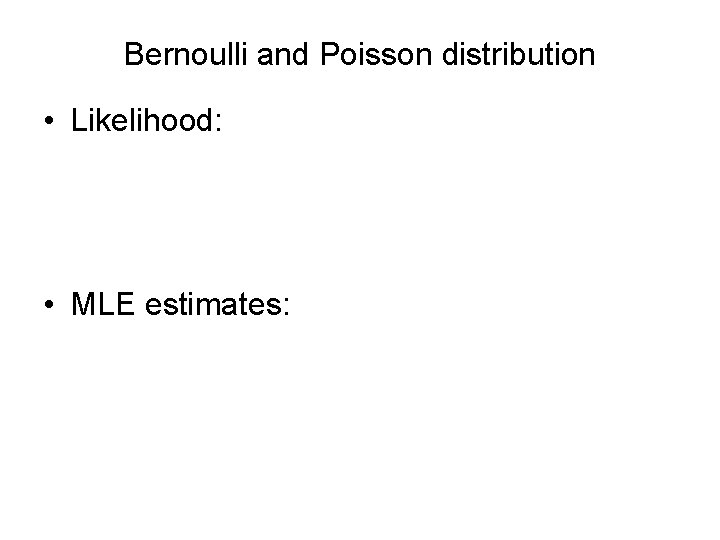
Bernoulli and Poisson distribution • Likelihood: • MLE estimates:

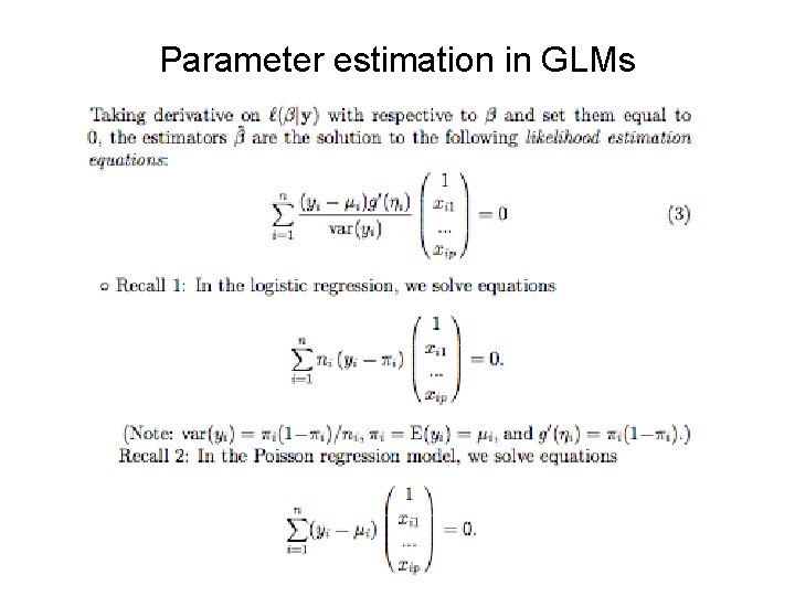
Parameter estimation in GLMs

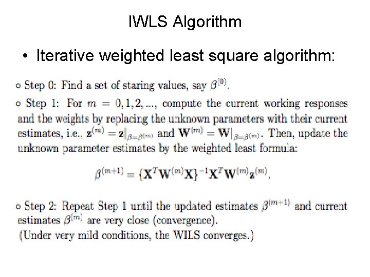
IWLS Algorithm • Iterative weighted least square algorithm: