Chapter 12 Systematic Risk and the Equity Risk

Chapter 12 Systematic Risk and the Equity Risk Premium

Chapter Outline 12. 1 12. 2 12. 3 12. 4 The Expected Return of a Portfolio The Volatility of a Portfolio Measuring Systematic Risk Putting it All Together: The Capital Asset Pricing Model

Learning Objectives �Calculate the expected return and volatility (standard deviation) of a portfolio �Understand the relation between systematic risk and the market portfolio �Measure systematic risk �Use the Capital Asset Pricing Model (CAPM) to compute the cost of equity capital for a stock

Review Chapter 11 • We started our exploration of the tradeoff between risk and return. We found that for large portfolios, while investors should expect to experience higher returns for higher risk, the same does not hold true for individual stocks. Stocks have both unsystematic, diversifiable risk and systematic, undiversifiable risk; only the systematic risk is rewarded with higher expected returns. With no reward for bearing unsystematic risk, rational investors should choose to diversify. • We learned the important role that portfolio play in reducing unsystematic risk. • It is important to understand how portfolio work and the implications for the return our investors expect on the stock of our company and the projects we undertake in that company.

12. 1 The Expected Return of a Portfolio �In Chapter 11 we found: �For large portfolios, investors expect higher returns for higher risk. �The same does not hold true for individual stocks. �Stocks have both unsystematic and systematic risk �only systematic risk is rewarded �rational investors should choose to diversify.

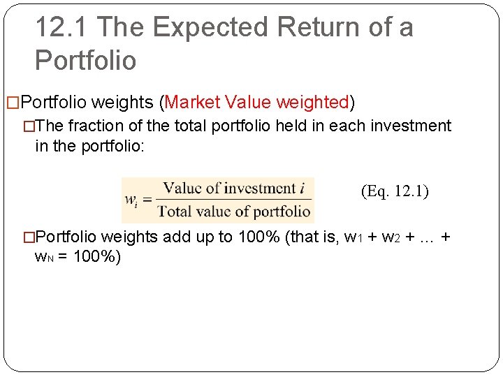
12. 1 The Expected Return of a Portfolio �Portfolio weights (Market Value weighted) �The fraction of the total portfolio held in each investment in the portfolio: (Eq. 12. 1) �Portfolio weights add up to 100% (that is, w 1 + w 2 + … + w. N = 100%)

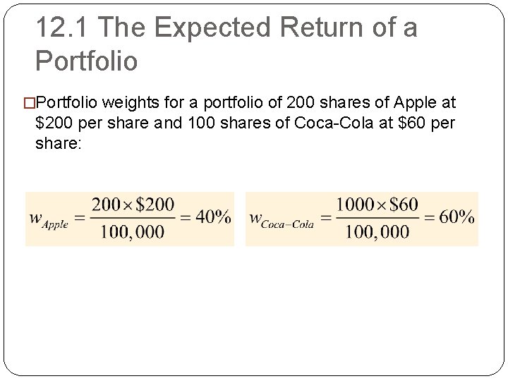
12. 1 The Expected Return of a Portfolio �Portfolio weights for a portfolio of 200 shares of Apple at $200 per share and 100 shares of Coca-Cola at $60 per share:

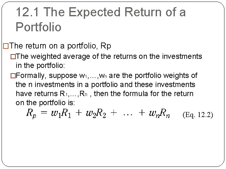
12. 1 The Expected Return of a Portfolio �The return on a portfolio, Rp �The weighted average of the returns on the investments in the portfolio: �Formally, suppose w 1, …, wn are the portfolio weights of the n investments in a portfolio and these investments have returns R 1, …, Rn , then the formula for the return on the portfolio is: (Eq. 12. 2)

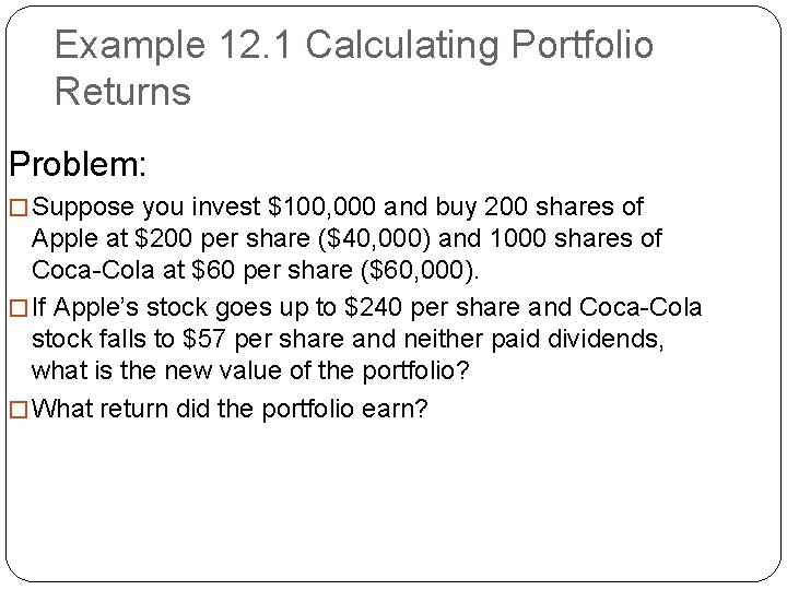
Example 12. 1 Calculating Portfolio Returns Problem: � Suppose you invest $100, 000 and buy 200 shares of Apple at $200 per share ($40, 000) and 1000 shares of Coca-Cola at $60 per share ($60, 000). � If Apple’s stock goes up to $240 per share and Coca-Cola stock falls to $57 per share and neither paid dividends, what is the new value of the portfolio? � What return did the portfolio earn?

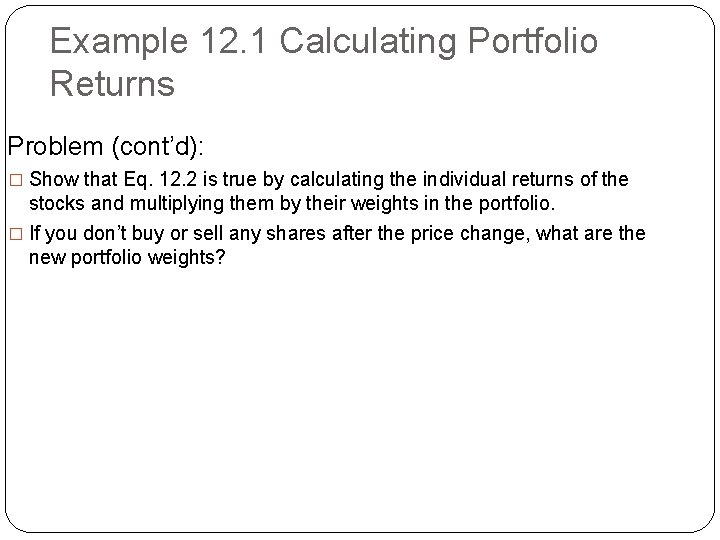
Example 12. 1 Calculating Portfolio Returns Problem (cont’d): � Show that Eq. 12. 2 is true by calculating the individual returns of the stocks and multiplying them by their weights in the portfolio. � If you don’t buy or sell any shares after the price change, what are the new portfolio weights?

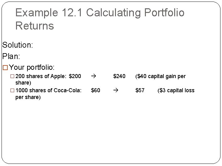
Example 12. 1 Calculating Portfolio Returns Solution: Plan: � Your portfolio: � 200 shares of Apple: $200 $240 ($40 capital gain per share) � 1000 shares of Coca-Cola: per share) $60 $57 ($3 capital loss

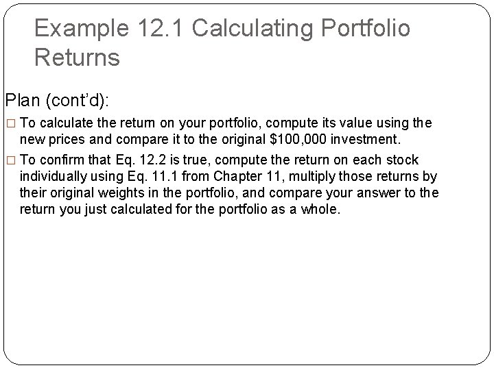
Example 12. 1 Calculating Portfolio Returns Plan (cont’d): � To calculate the return on your portfolio, compute its value using the new prices and compare it to the original $100, 000 investment. � To confirm that Eq. 12. 2 is true, compute the return on each stock individually using Eq. 11. 1 from Chapter 11, multiply those returns by their original weights in the portfolio, and compare your answer to the return you just calculated for the portfolio as a whole.

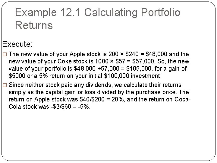
Example 12. 1 Calculating Portfolio Returns Execute: � The new value of your Apple stock is 200 × $240 = $48, 000 and the new value of your Coke stock is 1000 × $57 = $57, 000. So, the new value of your portfolio is $48, 000 +57, 000 = $105, 000, for a gain of $5000 or a 5% return on your initial $100, 000 investment. � Since neither stock paid any dividends, we calculate their returns simply as the capital gain or loss divided by the purchase price. The return on Apple stock was $40/$200 = 20%, and the return on Coca. Cola stock was -$3/$60 = -5%.

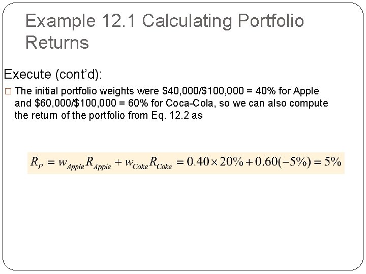
Example 12. 1 Calculating Portfolio Returns Execute (cont’d): � The initial portfolio weights were $40, 000/$100, 000 = 40% for Apple and $60, 000/$100, 000 = 60% for Coca-Cola, so we can also compute the return of the portfolio from Eq. 12. 2 as

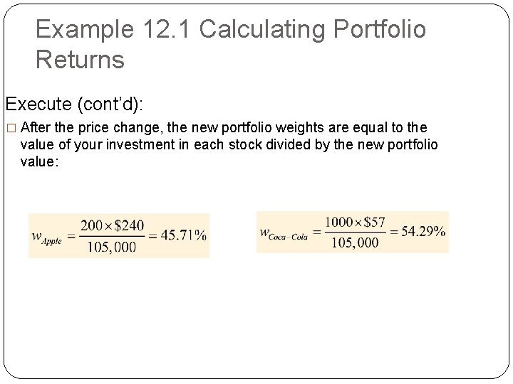
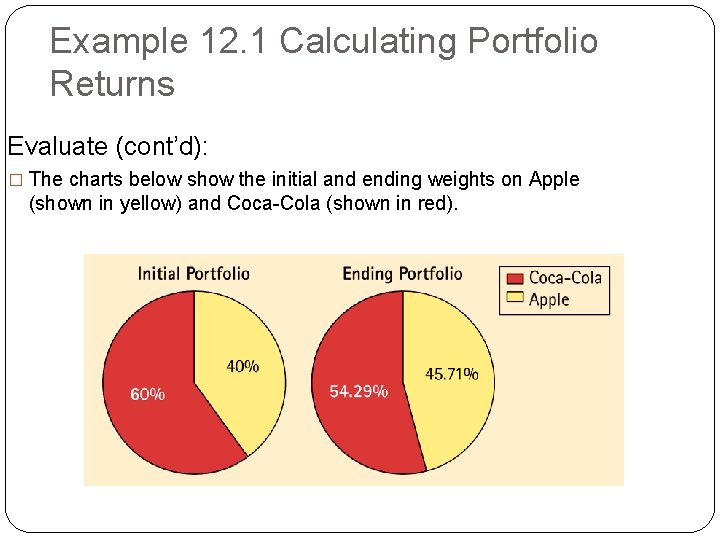
Example 12. 1 Calculating Portfolio Returns Execute (cont’d): � After the price change, the new portfolio weights are equal to the value of your investment in each stock divided by the new portfolio value:

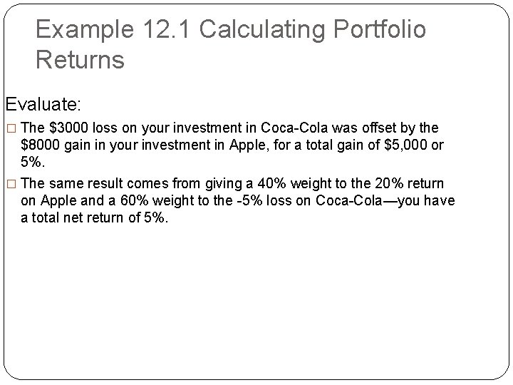
Example 12. 1 Calculating Portfolio Returns Evaluate: � The $3000 loss on your investment in Coca-Cola was offset by the $8000 gain in your investment in Apple, for a total gain of $5, 000 or 5%. � The same result comes from giving a 40% weight to the 20% return on Apple and a 60% weight to the -5% loss on Coca-Cola—you have a total net return of 5%.

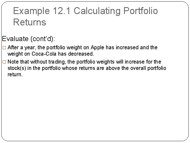
Example 12. 1 Calculating Portfolio Returns Evaluate (cont’d): � After a year, the portfolio weight on Apple has increased and the weight on Coca-Cola has decreased. � Note that without trading, the portfolio weights will increase for the stock(s) in the portfolio whose returns are above the overall portfolio return.

Example 12. 1 Calculating Portfolio Returns Evaluate (cont’d): � The charts below show the initial and ending weights on Apple (shown in yellow) and Coca-Cola (shown in red).

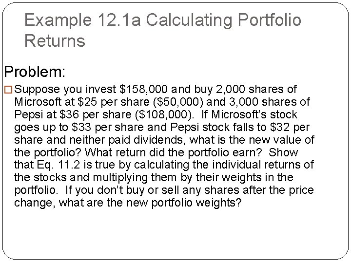
Example 12. 1 a Calculating Portfolio Returns Problem: � Suppose you invest $158, 000 and buy 2, 000 shares of Microsoft at $25 per share ($50, 000) and 3, 000 shares of Pepsi at $36 per share ($108, 000). If Microsoft’s stock goes up to $33 per share and Pepsi stock falls to $32 per share and neither paid dividends, what is the new value of the portfolio? What return did the portfolio earn? Show that Eq. 11. 2 is true by calculating the individual returns of the stocks and multiplying them by their weights in the portfolio. If you don’t buy or sell any shares after the price change, what are the new portfolio weights?

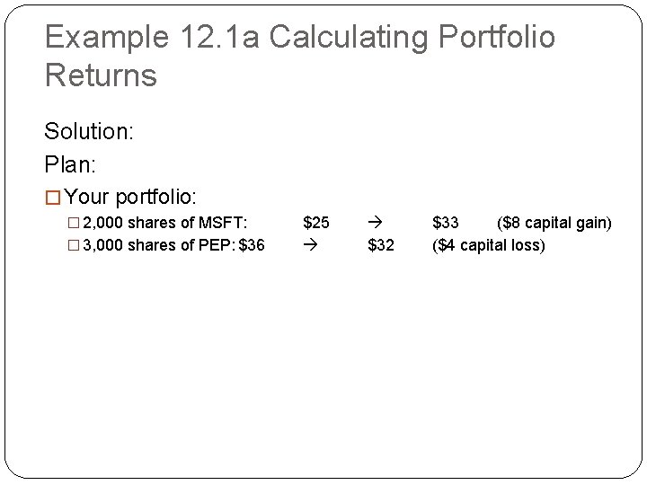
Example 12. 1 a Calculating Portfolio Returns Solution: Plan: � Your portfolio: � 2, 000 shares of MSFT: � 3, 000 shares of PEP: $36 $25 $32 $33 ($8 capital gain) ($4 capital loss)

Example 12. 1 a Calculating Portfolio Returns Plan (cont’d): � To calculate the return on your portfolio, compute its value using the new prices and compare it to the original $158, 000 investment. � To confirm that Eq. 12. 2 is true, compute the return on each stock individually using Eq. 11. 1 from Chapter 11, multiply those returns by their original weights in the portfolio, and compare your answer to the return you just calculated for the portfolio as a whole.

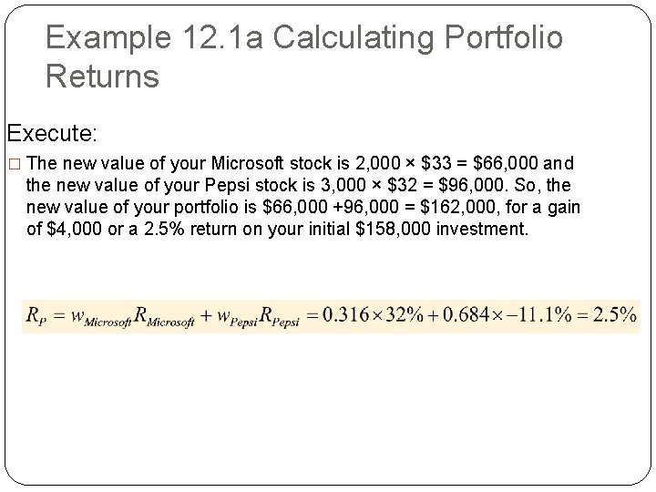
Example 12. 1 a Calculating Portfolio Returns Execute: � The new value of your Microsoft stock is 2, 000 × $33 = $66, 000 and the new value of your Pepsi stock is 3, 000 × $32 = $96, 000. So, the new value of your portfolio is $66, 000 +96, 000 = $162, 000, for a gain of $4, 000 or a 2. 5% return on your initial $158, 000 investment.

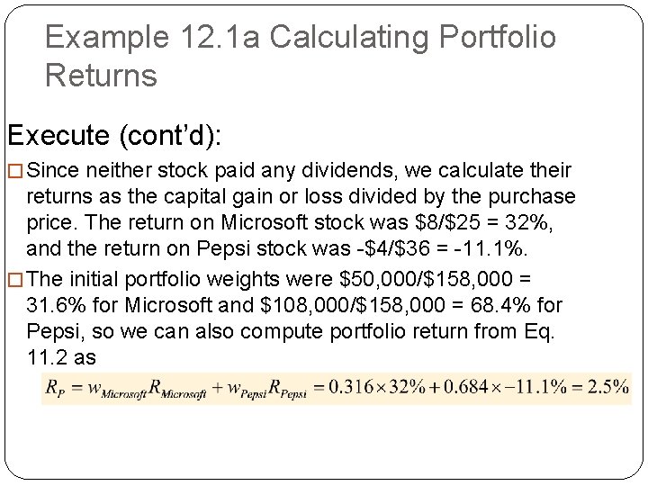
Example 12. 1 a Calculating Portfolio Returns Execute (cont’d): � Since neither stock paid any dividends, we calculate their returns as the capital gain or loss divided by the purchase price. The return on Microsoft stock was $8/$25 = 32%, and the return on Pepsi stock was -$4/$36 = -11. 1%. � The initial portfolio weights were $50, 000/$158, 000 = 31. 6% for Microsoft and $108, 000/$158, 000 = 68. 4% for Pepsi, so we can also compute portfolio return from Eq. 11. 2 as

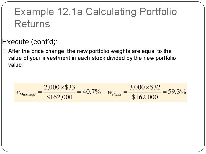
Example 12. 1 a Calculating Portfolio Returns Execute (cont’d): � After the price change, the new portfolio weights are equal to the value of your investment in each stock divided by the new portfolio value:

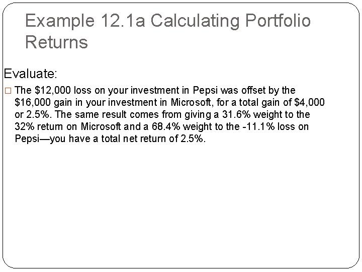
Example 12. 1 a Calculating Portfolio Returns Evaluate: � The $12, 000 loss on your investment in Pepsi was offset by the $16, 000 gain in your investment in Microsoft, for a total gain of $4, 000 or 2. 5%. The same result comes from giving a 31. 6% weight to the 32% return on Microsoft and a 68. 4% weight to the -11. 1% loss on Pepsi—you have a total net return of 2. 5%.

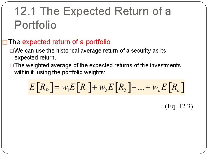
12. 1 The Expected Return of a Portfolio � The expected return of a portfolio �We can use the historical average return of a security as its expected return. �The weighted average of the expected returns of the investments within it, using the portfolio weights: (Eq. 12. 3)

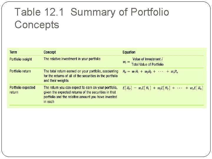
Table 12. 1 Summary of Portfolio Concepts

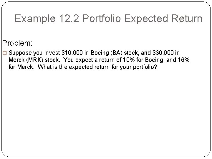
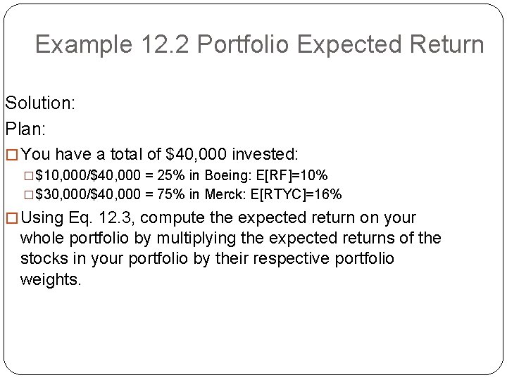
Example 12. 2 Portfolio Expected Return Problem: � Suppose you invest $10, 000 in Boeing (BA) stock, and $30, 000 in Merck (MRK) stock. You expect a return of 10% for Boeing, and 16% for Merck. What is the expected return for your portfolio?

Example 12. 2 Portfolio Expected Return Solution: Plan: � You have a total of $40, 000 invested: �$10, 000/$40, 000 = 25% in Boeing: E[RF]=10% �$30, 000/$40, 000 = 75% in Merck: E[RTYC]=16% � Using Eq. 12. 3, compute the expected return on your whole portfolio by multiplying the expected returns of the stocks in your portfolio by their respective portfolio weights.

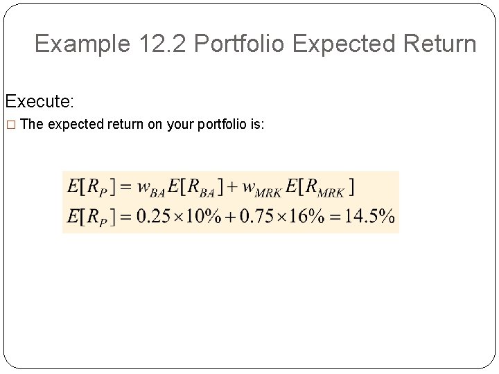
Example 12. 2 Portfolio Expected Return Execute: � The expected return on your portfolio is:

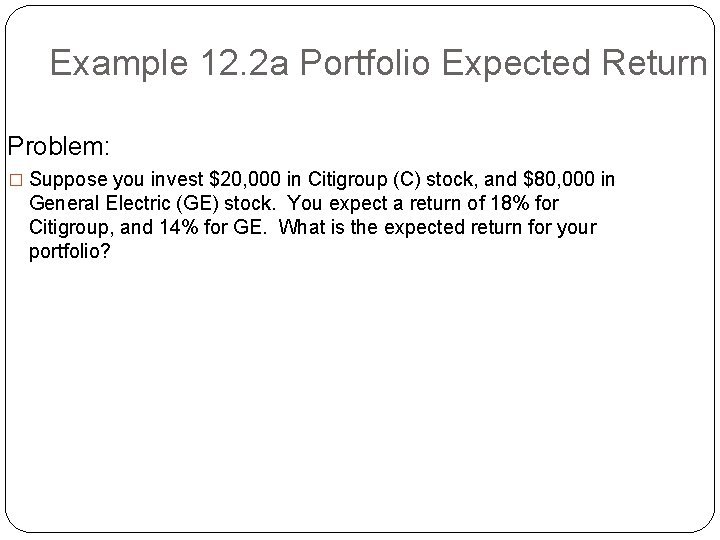
Example 12. 2 a Portfolio Expected Return Problem: � Suppose you invest $20, 000 in Citigroup (C) stock, and $80, 000 in General Electric (GE) stock. You expect a return of 18% for Citigroup, and 14% for GE. What is the expected return for your portfolio?

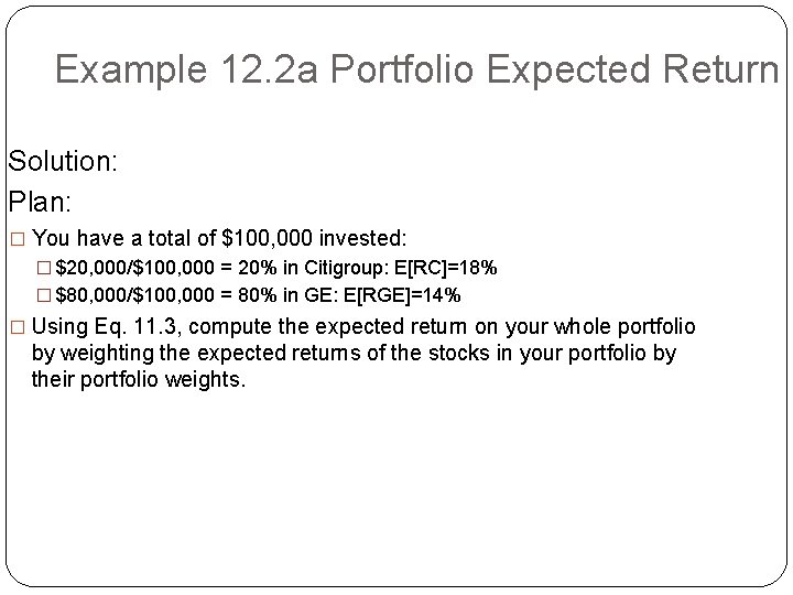
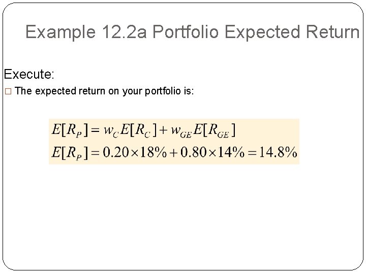
Example 12. 2 a Portfolio Expected Return Solution: Plan: � You have a total of $100, 000 invested: � $20, 000/$100, 000 = 20% in Citigroup: E[RC]=18% � $80, 000/$100, 000 = 80% in GE: E[RGE]=14% � Using Eq. 11. 3, compute the expected return on your whole portfolio by weighting the expected returns of the stocks in your portfolio by their portfolio weights.

Example 12. 2 a Portfolio Expected Return Execute: � The expected return on your portfolio is:

12. 2 The Volatility of a Portfolio �Investors care about return, but also risk �When we combine stocks in a portfolio, some risk is eliminated through diversification. �Remaining risk depends upon the degree to which the stocks share common risk. �The volatility of a portfolio is the total risk, measured as standard deviation, of the portfolio.

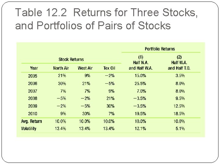
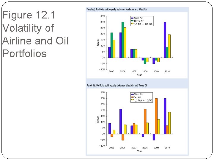
12. 2 The Volatility of a Portfolio �Table 12. 2 shows returns for three hypothetical stocks, along with their average returns and volatilities. �Note that while three stocks have the same volatility and average return, the pattern of returns differs. �When the airline stocks performed well, the oil stock did poorly, and when the airlines did poorly, the oil stock did well.

Table 12. 2 Returns for Three Stocks, and Portfolios of Pairs of Stocks

12. 2 The Volatility of a Portfolio �Table 12. 2 shows returns for two portfolios: �An equal investment in the two airlines, North Air and West Air. �An equal investment in West Air and Tex Oil. �Average return of both portfolios is equal to the average return of the stocks �Volatilities (standard deviations) are very different.

Figure 12. 1 Volatility of Airline and Oil Portfolios

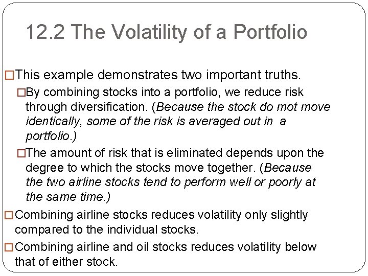
12. 2 The Volatility of a Portfolio �This example demonstrates two important truths. �By combining stocks into a portfolio, we reduce risk through diversification. (Because the stock do mot move identically, some of the risk is averaged out in a portfolio. ) �The amount of risk that is eliminated depends upon the degree to which the stocks move together. (Because the two airline stocks tend to perform well or poorly at the same time. ) � Combining airline stocks reduces volatility only slightly compared to the individual stocks. � Combining airline and oil stocks reduces volatility below that of either stock.

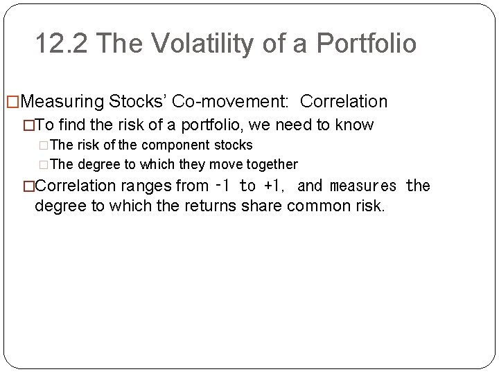
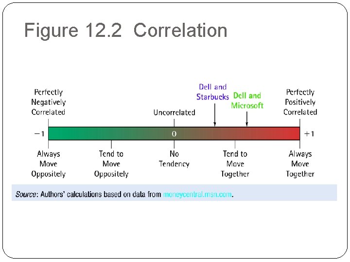
12. 2 The Volatility of a Portfolio �Measuring Stocks’ Co-movement: Correlation �To find the risk of a portfolio, we need to know �The risk of the component stocks �The degree to which they move together �Correlation ranges from ‑ 1 to +1, and measures the degree to which the returns share common risk.

Figure 12. 2 Correlation

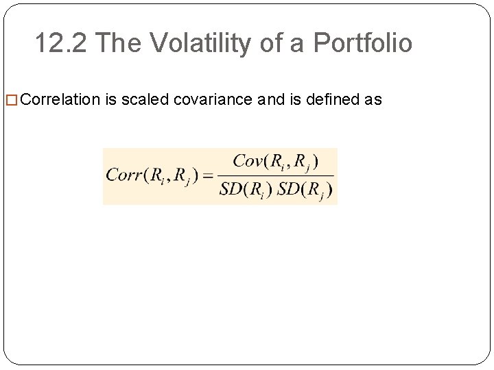
12. 2 The Volatility of a Portfolio � Correlation is scaled covariance and is defined as

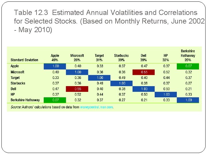
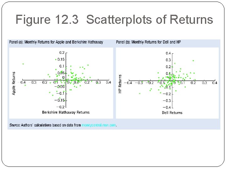
12. 2 The Volatility of a Portfolio �Stock returns tend to move together if they are affected similarly by economic events. �Stocks in the same industry tend to have more highly correlated returns than stocks in different industries. �Table 12. 3 shows several stocks’ �Volatility of individual stock returns �Correlation between them �The table can be read across rows or down columns.

Table 12. 3 Estimated Annual Volatilities and Correlations for Selected Stocks. (Based on Monthly Returns, June 2002 - May 2010)

Figure 12. 3 Scatterplots of Returns

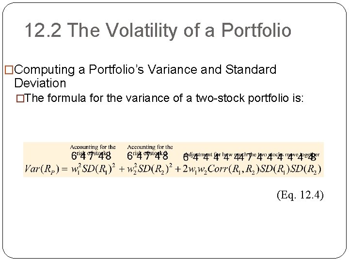
12. 2 The Volatility of a Portfolio �Computing a Portfolio’s Variance and Standard Deviation �The formula for the variance of a two-stock portfolio is: (Eq. 12. 4)

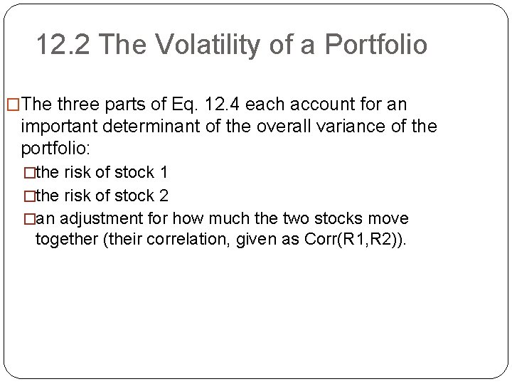
12. 2 The Volatility of a Portfolio �The three parts of Eq. 12. 4 each account for an important determinant of the overall variance of the portfolio: �the risk of stock 1 �the risk of stock 2 �an adjustment for how much the two stocks move together (their correlation, given as Corr(R 1, R 2)).

12. 2 The Volatility of a Portfolio �Expected return of a portfolio is equal to the weighted average expected return of its stocks. �Risk of the portfolio is lower than the weighted average of the individual stocks’ volatility, unless all the stocks all have perfect positive correlation with each other �It’s clear that we can eliminate some volatility by Diversification.

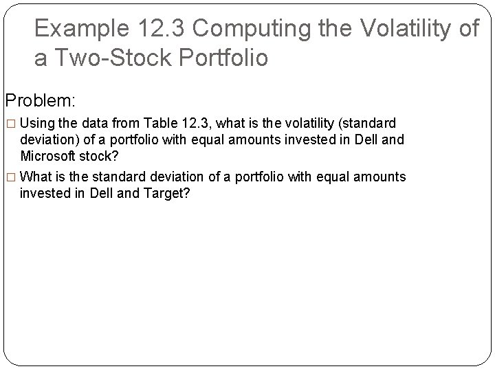
Example 12. 3 Computing the Volatility of a Two-Stock Portfolio Problem: � Using the data from Table 12. 3, what is the volatility (standard deviation) of a portfolio with equal amounts invested in Dell and Microsoft stock? � What is the standard deviation of a portfolio with equal amounts invested in Dell and Target?

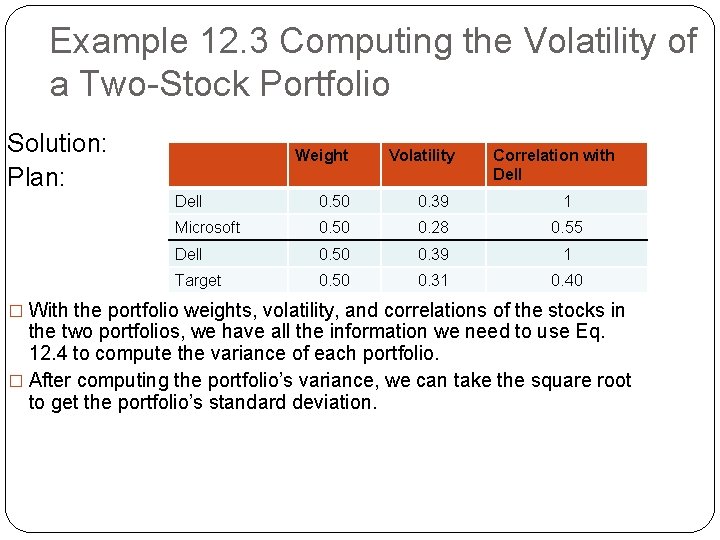
Example 12. 3 Computing the Volatility of a Two-Stock Portfolio Solution: Plan: Weight Volatility Correlation with Dell 0. 50 0. 39 1 Microsoft 0. 50 0. 28 0. 55 Dell 0. 50 0. 39 1 Target 0. 50 0. 31 0. 40 � With the portfolio weights, volatility, and correlations of the stocks in the two portfolios, we have all the information we need to use Eq. 12. 4 to compute the variance of each portfolio. � After computing the portfolio’s variance, we can take the square root to get the portfolio’s standard deviation.

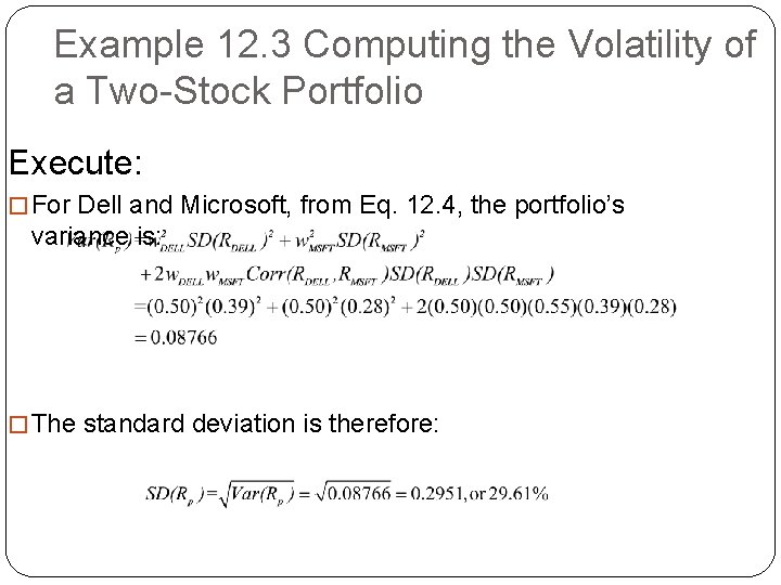
Example 12. 3 Computing the Volatility of a Two-Stock Portfolio Execute: � For Dell and Microsoft, from Eq. 12. 4, the portfolio’s variance is: � The standard deviation is therefore:

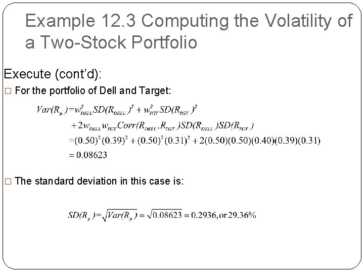
Example 12. 3 Computing the Volatility of a Two-Stock Portfolio Execute (cont’d): � For the portfolio of Dell and Target: � The standard deviation in this case is:

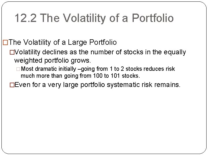
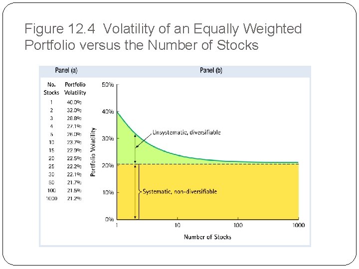
12. 2 The Volatility of a Portfolio �The Volatility of a Large Portfolio �Volatility declines as the number of stocks in the equally weighted portfolio grows. �Most dramatic initially –going from 1 to 2 stocks reduces risk much more than going from 100 to 101 stocks. �Even for a very large portfolio systematic risk remains.

Figure 12. 4 Volatility of an Equally Weighted Portfolio versus the Number of Stocks

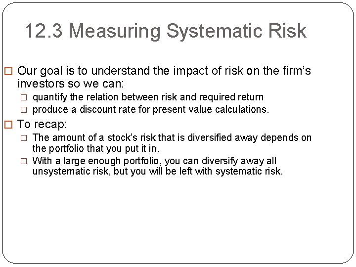
12. 3 Measuring Systematic Risk � Our goal is to understand the impact of risk on the firm’s investors so we can: � quantify the relation between risk and required return � produce a discount rate for present value calculations. � To recap: � The amount of a stock’s risk that is diversified away depends on the portfolio that you put it in. � With a large enough portfolio, you can diversify away all unsystematic risk, but you will be left with systematic risk.

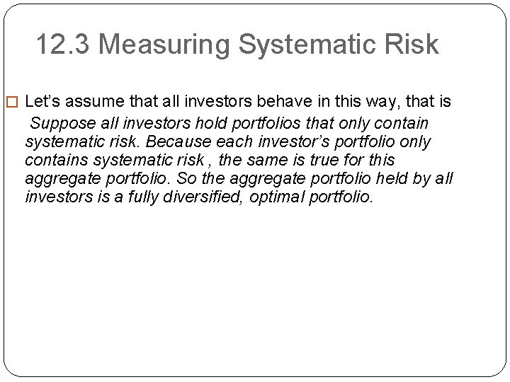
12. 3 Measuring Systematic Risk � Let’s assume that all investors behave in this way, that is Suppose all investors hold portfolios that only contain systematic risk. Because each investor’s portfolio only contains systematic risk , the same is true for this aggregate portfolio. So the aggregate portfolio held by all investors is a fully diversified, optimal portfolio.

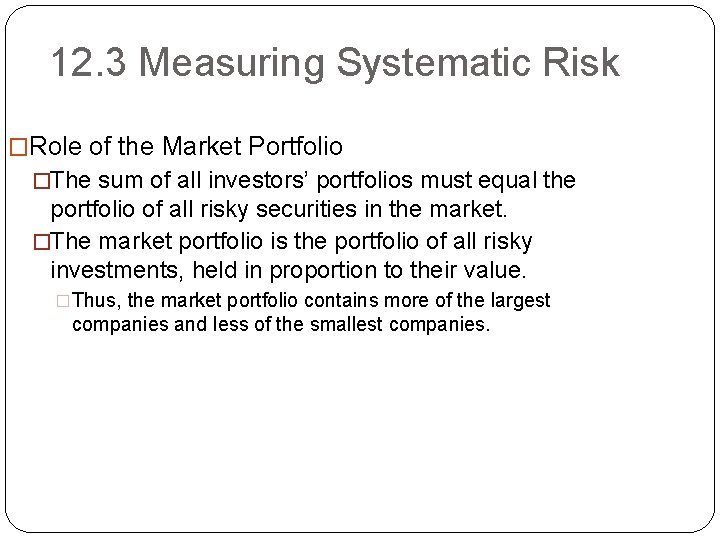
12. 3 Measuring Systematic Risk �Role of the Market Portfolio �The sum of all investors’ portfolios must equal the portfolio of all risky securities in the market. �The market portfolio is the portfolio of all risky investments, held in proportion to their value. �Thus, the market portfolio contains more of the largest companies and less of the smallest companies.

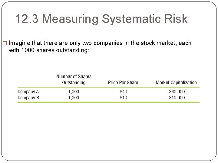
12. 3 Measuring Systematic Risk � Imagine that there are only two companies in the stock market, each with 1000 shares outstanding:

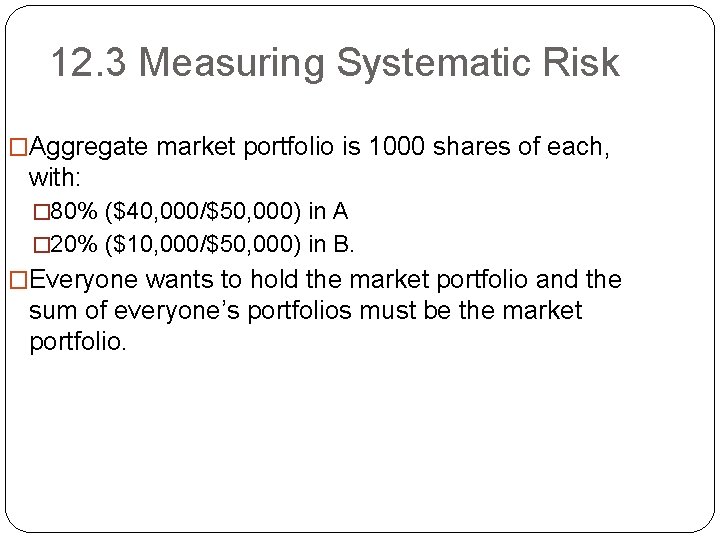
12. 3 Measuring Systematic Risk �Aggregate market portfolio is 1000 shares of each, with: � 80% ($40, 000/$50, 000) in A � 20% ($10, 000/$50, 000) in B. �Everyone wants to hold the market portfolio and the sum of everyone’s portfolios must be the market portfolio.

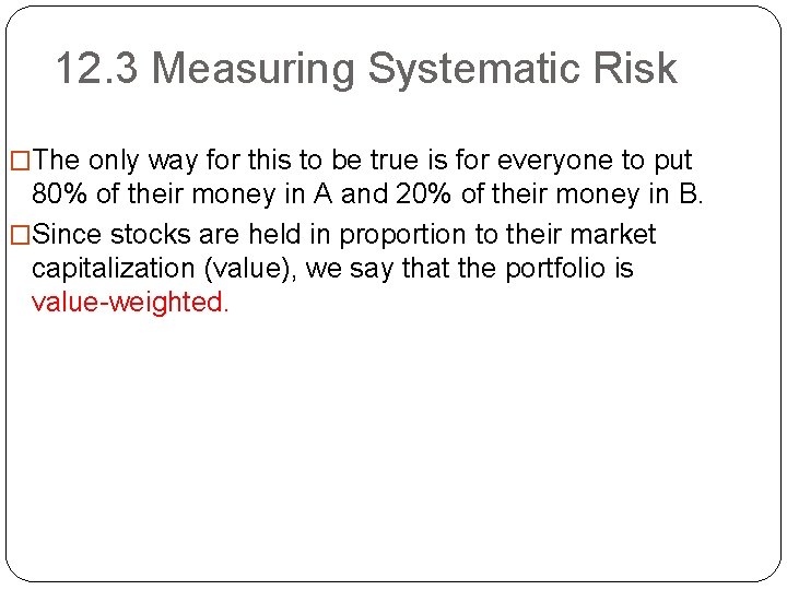
12. 3 Measuring Systematic Risk �The only way for this to be true is for everyone to put 80% of their money in A and 20% of their money in B. �Since stocks are held in proportion to their market capitalization (value), we say that the portfolio is value-weighted.

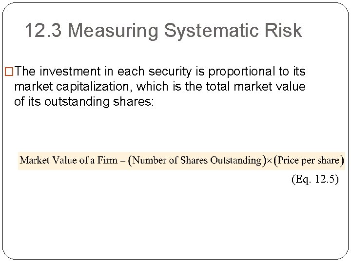
12. 3 Measuring Systematic Risk �The investment in each security is proportional to its market capitalization, which is the total market value of its outstanding shares: (Eq. 12. 5)

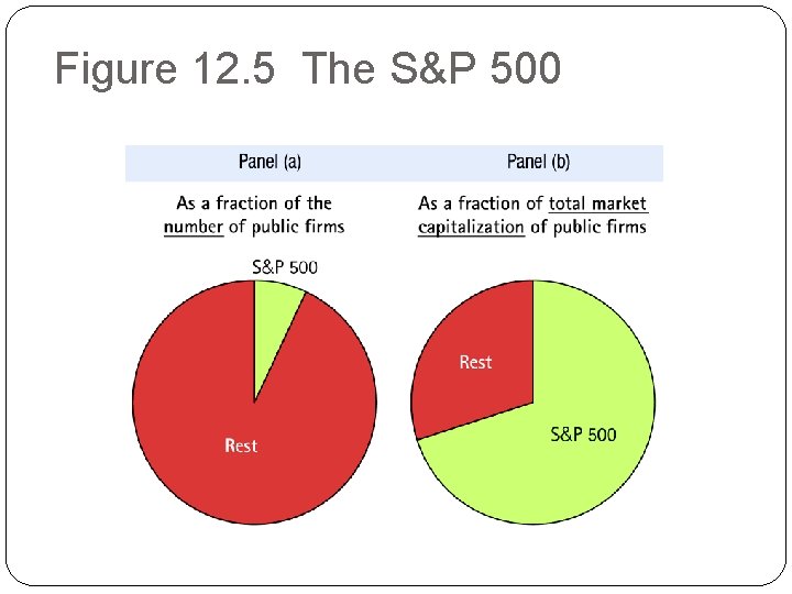
12. 3 Measuring Systematic Risk �Stock Market Indexes as the Market Portfolio �In practice we use a market proxy—a portfolio whose return should track the underlying, unobservable market portfolio. �The most common proxy portfolios are market indexes. �A market index reports the value of a particular portfolio. � Dow Jones Industrial Average � S&P 500

Figure 12. 5 The S&P 500

12. 3 Measuring Systematic Risk �Market Risk and Beta �We compare a stock’s historical returns to the market’s historical returns to determine a stock’s beta (β) �The sensitivity of an investment to fluctuations in the market portfolio. �Use excess returns – security return less the risk-free rate �The percentage change in the stock’s return that we expect for each 1% change in the market’s return

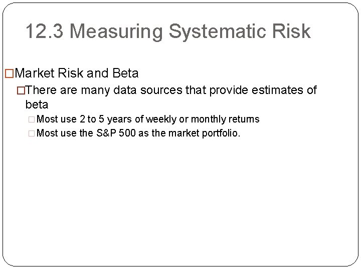
12. 3 Measuring Systematic Risk �Market Risk and Beta �There are many data sources that provide estimates of beta �Most use 2 to 5 years of weekly or monthly returns �Most use the S&P 500 as the market portfolio.

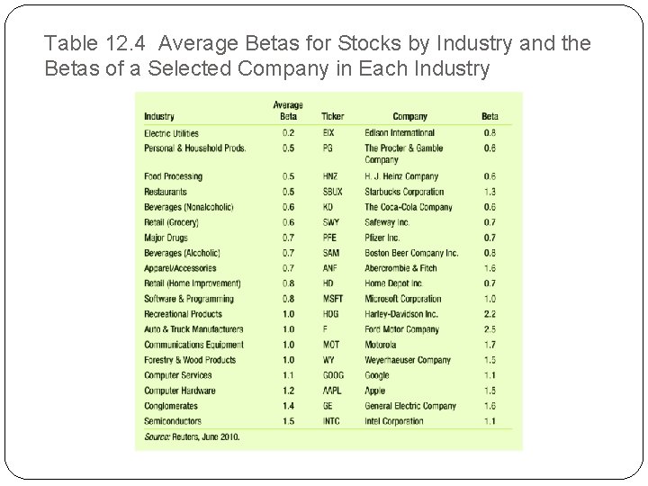
Table 12. 4 Average Betas for Stocks by Industry and the Betas of a Selected Company in Each Industry

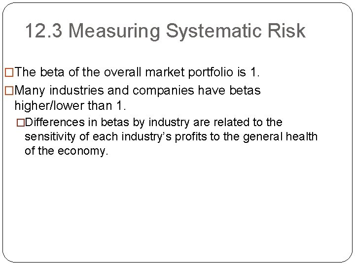
12. 3 Measuring Systematic Risk �The beta of the overall market portfolio is 1. �Many industries and companies have betas higher/lower than 1. �Differences in betas by industry are related to the sensitivity of each industry’s profits to the general health of the economy.

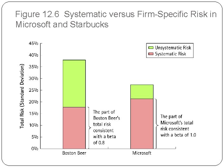
Figure 12. 6 Systematic versus Firm-Specific Risk in Microsoft and Starbucks

12. 3 Measuring Systematic Risk �Estimating Beta from Historical Returns �Beta is the expected percentage change in the excess return of the security for a 1% change in the excess return of the market portfolio. �The amount by which risks that affect the overall market are amplified or dampened in a given stock or investment.

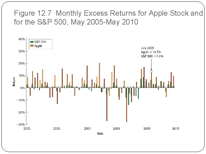
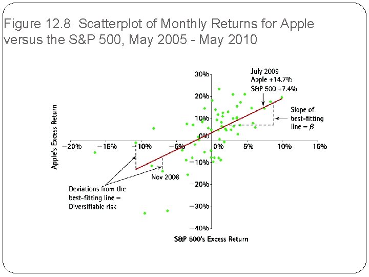
12. 3 Measuring Systematic Risk �Estimating Beta from Historical Returns �Apple’s stock for example (Figure 12. 7): �The overall tendency is for Apple to have a high return when the market is up and a low return when the market is down. �Apple tends to move in the same direction as the market, but its movements are larger. �The pattern suggests that Apple’s beta is greater than one.

Figure 12. 7 Monthly Excess Returns for Apple Stock and for the S&P 500, May 2005 -May 2010

12. 3 Measuring Systematic Risk �In practice, we use linear regression to estimate the relation. �The output is the best-fitting line that represents the historical relation between the stock and the market. �The slope of this line is our estimate of beta. �Tells us how much the stock’s excess return changed for a 1% change in the market’s excess return.

Figure 12. 8 Scatterplot of Monthly Returns for Apple versus the S&P 500, May 2005 - May 2010

12. 4 Putting It All Together: The Capital Asset Pricing Model �One of our goals in this chapter is to compute the cost of equity capital �The best available expected return offered in the market on a similar investment. �To compute the cost of equity capital, we need to know the relation between the stock’s risk and its expected return.

12. 4 Putting It All Together: The Capital Asset Pricing Model �The CAPM Equation Relating Risk to Expected Return �Only systematic risk determines expected returns �Firm-specific risk is diversifiable and does not warrant extra return.

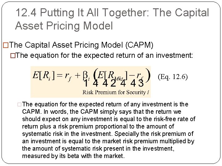
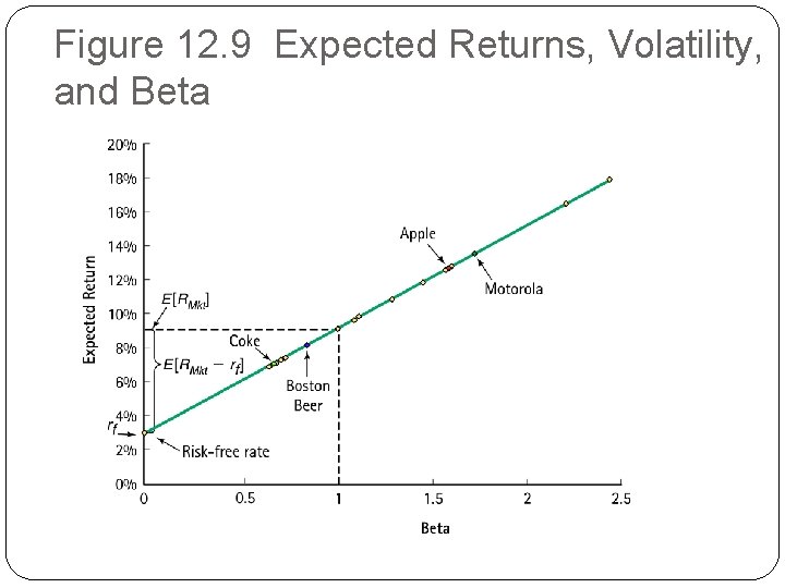
12. 4 Putting It All Together: The Capital Asset Pricing Model �The CAPM Equation Relating Risk to Expected Return �The expected return on any investment comes from two components: �A risk-free rate of return to compensate for inflation and the time value of money, even with no risk of losing money. �A risk premium that varies with the systematic risk �Expected Return = Risk-free rate + Risk Premium for Systematic Risk(per unit of beta) �We know that the market portfolio has exactly one unit of systematic risk. So, a natural estimate of the risk premium per unit of systematic risk is the historical average excess return on the market portfolio, also known as the market or equity risk premium.

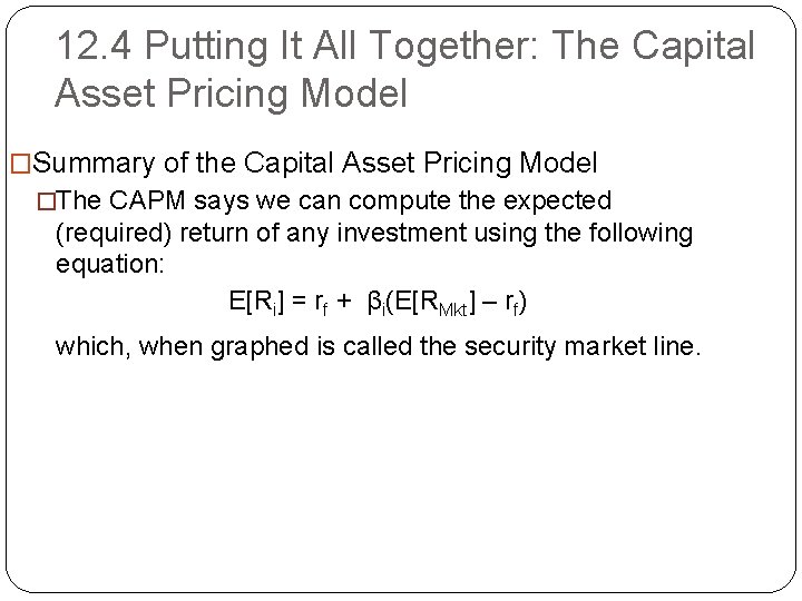
12. 4 Putting It All Together: The Capital Asset Pricing Model �The Capital Asset Pricing Model (CAPM) �The equation for the expected return of an investment: (Eq. 12. 6) �The equation for the expected return of any investment is the CAPM. In words, the CAPM simply says that the return we should expect on any investment is equal to the risk-free rate of return plus a risk premium proportional to the amount of systematic risk in the investment. Specially the risk premium of an investment is equal to the market risk premium multiplied by the amount of systematic risk present in the investment, measured by its beta with the market.

12. 4 Putting It All Together: The Capital Asset Pricing Model � The CAPM says that the expected return on any investment is equal to the risk-free rate of return plus a risk premium proportional to the amount of systematic risk in the investment. �The risk premium is equal to the market risk premium times the amount of systematic risk present in the investment, measured by its beta (βi). �Investors will not invest in this security unless they can expect at least the return given in CAPM, we also call this return the investment’s required return.

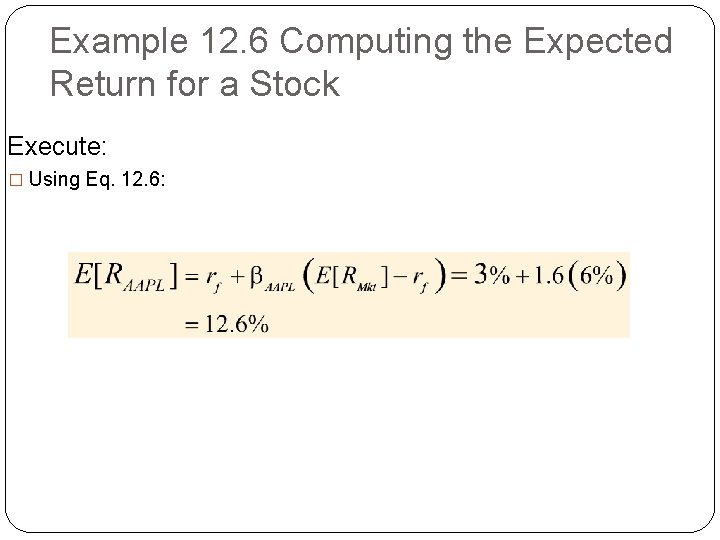
Example 12. 6 Computing the Expected Return for a Stock Problem: � Suppose the risk-free return is 3% and you measure the market risk premium to be 6%. Apple has a beta of 1. 6. According to the CAPM, what is its expected return?

Example 12. 6 Computing the Expected Return for a Stock Solution: Plan: � We can use Eq 12. 6 to compute the expected return according to the CAPM. For that equation, we will need the market risk premium, the risk-free return, and the stock’s beta. We have all of these inputs, so we are ready to go.

Example 12. 6 Computing the Expected Return for a Stock Execute: � Using Eq. 12. 6:

Example 12. 6 Computing the Expected Return for a Stock Evaluate: � Because of Apple’s beta of 1. 6, investors will require a risk premium of 9. 6% over the risk-free rate for investments in its stock to compensate for the systematic risk of Apple stock. This leads to a total expected return of 12. 6%.

12. 4 Putting It All Together: The Capital Asset Pricing Model �The Security Market Line �The CAPM implies a linear relation between a stock’s beta and its expected return. �This line is graphed in Figure 12. 9(b) as the line through the risk-free investment (with a beta of zero) and the market (with a beta of one); it is called the security market line (SML).

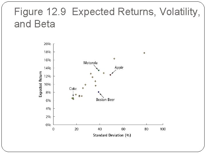
12. 4 Putting It All Together: The Capital Asset Pricing Model �The Security Market Line �Recall that there is no clear relation between a stock’s standard deviation (volatility) and its expected return �The relation between risk and return for individual securities is only evident when we measure market risk rather than total risk.

Figure 12. 9 Expected Returns, Volatility, and Beta

Figure 12. 9 Expected Returns, Volatility, and Beta

Example 12. 7 A Negative Beta Stock Problem: � Suppose the stock of Bankruptcy Auction Services, Inc. (BAS) has a negative beta of -0. 30. How does its expected return compare to the risk-free rate, according to the CAPM? Does your result make sense?

Example 12. 7 A Negative Beta Stock Evaluate: � This result seems odd—why would investors be willing to accept a 2. 2% expected return on this stock when they can invest in a safe investment and earn 4%? � The answer is that a savvy investor will not hold BAS alone; instead, the investor will hold it in combination with other securities as part of a well-diversified portfolio. � These other securities will tend to rise and fall with the market.

Example 12. 7 A Negative Beta Stock Evaluate (cont’d): � But because BAS has a negative beta, its correlation with the market is negative, which means that BAS tends to perform well when the rest of the market is doing poorly. � Therefore, by holding BAS, an investor can reduce the overall market risk of the portfolio. In a sense, BAS is “recession insurance” for a portfolio, and investors will pay for this insurance by accepting a lower return.

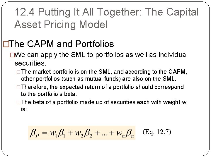
12. 4 Putting It All Together: The Capital Asset Pricing Model �The CAPM and Portfolios �We can apply the SML to portfolios as well as individual securities. �The market portfolio is on the SML, and according to the CAPM, other portfolios (such as mutual funds) are also on the SML. �Therefore, the expected return of a portfolio should correspond to the portfolio’s beta. �The beta of a portfolio made up of securities each with weight wi is: (Eq. 12. 7)

Example 12. 8 The Expected Return of a Portfolio Problem: � Suppose drug-maker Pfizer (PFE) has a beta of 0. 7, whereas the beta of Google (GOOG) is 1. 1. If the risk free interest rate is 3% and the market risk premium is 6%, what is the expected return of an equally weighted portfolio of Pfizer and Google, according to the CAPM?

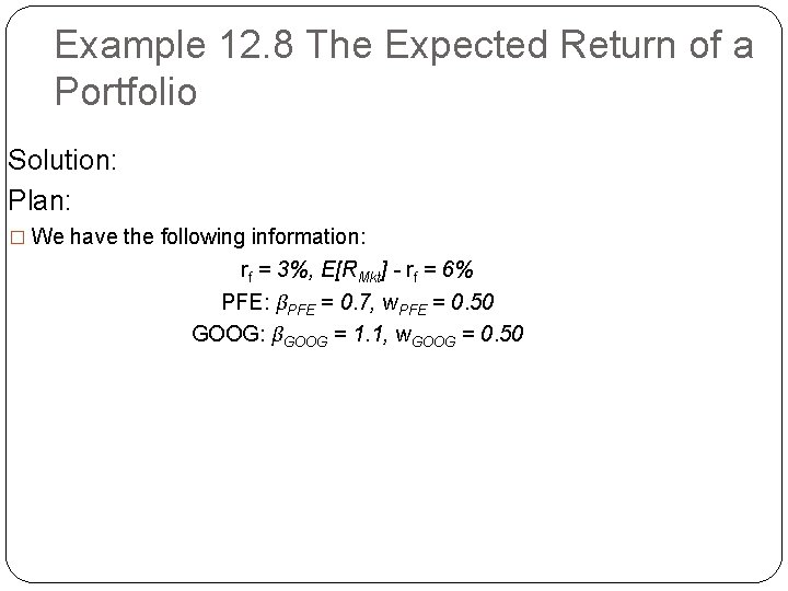
Example 12. 8 The Expected Return of a Portfolio Solution: Plan: � We have the following information: rf = 3%, E[RMkt] - rf = 6% PFE: βPFE = 0. 7, w. PFE = 0. 50 GOOG: βGOOG = 1. 1, w. GOOG = 0. 50

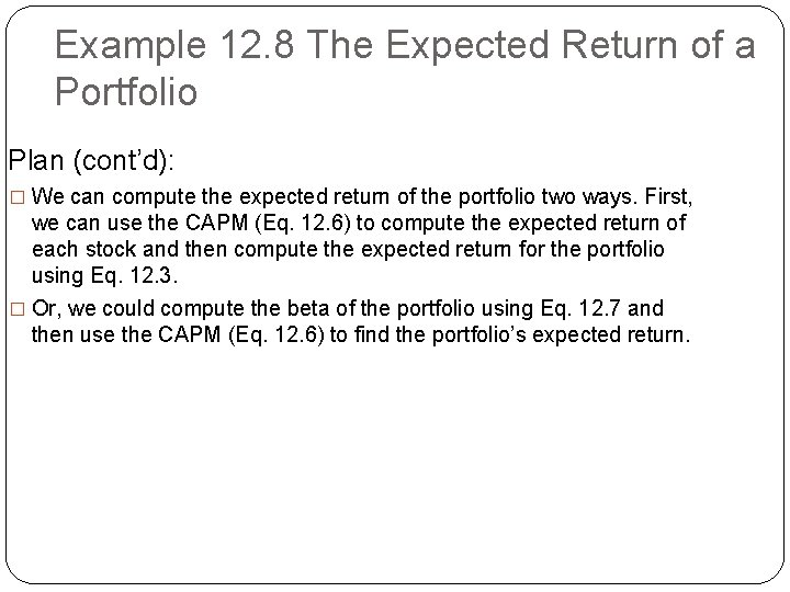
Example 12. 8 The Expected Return of a Portfolio Plan (cont’d): � We can compute the expected return of the portfolio two ways. First, we can use the CAPM (Eq. 12. 6) to compute the expected return of each stock and then compute the expected return for the portfolio using Eq. 12. 3. � Or, we could compute the beta of the portfolio using Eq. 12. 7 and then use the CAPM (Eq. 12. 6) to find the portfolio’s expected return.

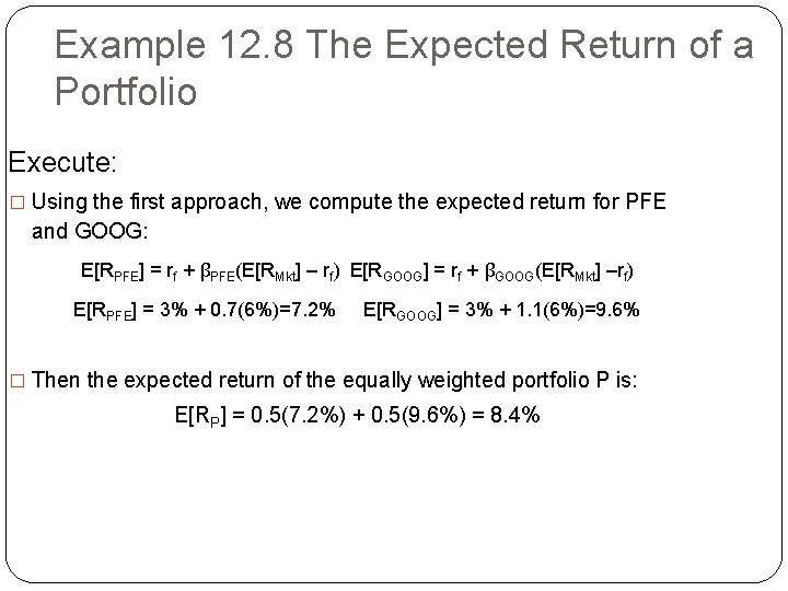
Example 12. 8 The Expected Return of a Portfolio Execute: � Using the first approach, we compute the expected return for PFE and GOOG: E[RPFE] = rf + βPFE(E[RMkt] – rf) E[RGOOG] = rf + βGOOG(E[RMkt] –rf) E[RPFE] = 3% + 0. 7(6%)=7. 2% E[RGOOG] = 3% + 1. 1(6%)=9. 6% � Then the expected return of the equally weighted portfolio P is: E[RP] = 0. 5(7. 2%) + 0. 5(9. 6%) = 8. 4%

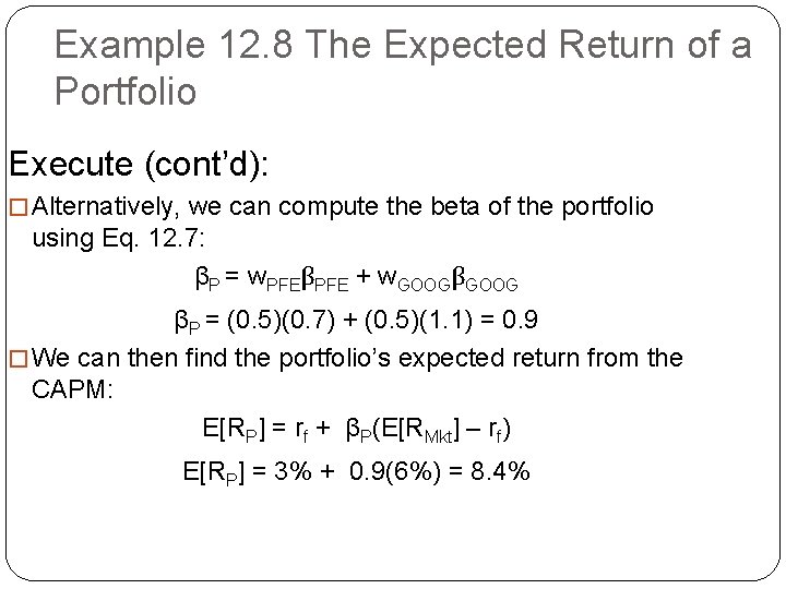
Example 12. 8 The Expected Return of a Portfolio Execute (cont’d): � Alternatively, we can compute the beta of the portfolio using Eq. 12. 7: βP = w. PFEβPFE + w. GOOGβGOOG βP = (0. 5)(0. 7) + (0. 5)(1. 1) = 0. 9 � We can then find the portfolio’s expected return from the CAPM: E[RP] = rf + βP(E[RMkt] – rf) E[RP] = 3% + 0. 9(6%) = 8. 4%

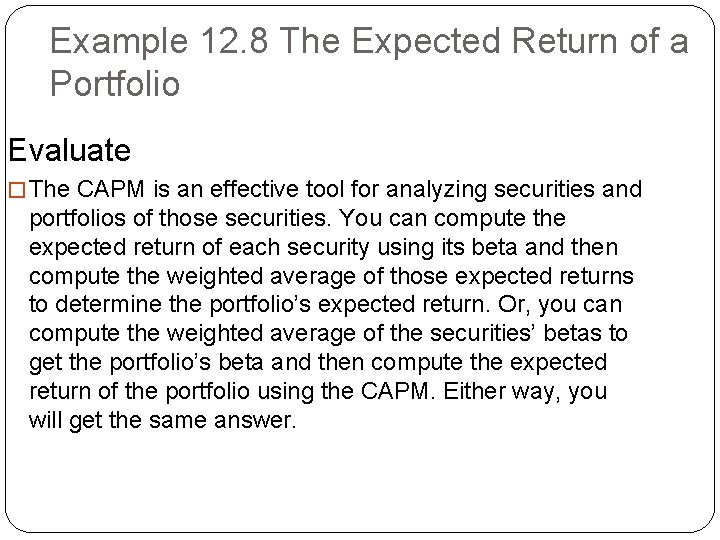
Example 12. 8 The Expected Return of a Portfolio Evaluate � The CAPM is an effective tool for analyzing securities and portfolios of those securities. You can compute the expected return of each security using its beta and then compute the weighted average of those expected returns to determine the portfolio’s expected return. Or, you can compute the weighted average of the securities’ betas to get the portfolio’s beta and then compute the expected return of the portfolio using the CAPM. Either way, you will get the same answer.

12. 4 Putting It All Together: The Capital Asset Pricing Model �Summary of the Capital Asset Pricing Model �Investors require a risk premium proportional to the amount of systematic risk they are bearing. �We can measure systematic risk using beta (β) �The most common way to estimate beta is to use linear regression – the slope of the line is the stock’s beta.

12. 4 Putting It All Together: The Capital Asset Pricing Model �Summary of the Capital Asset Pricing Model �The CAPM says we can compute the expected (required) return of any investment using the following equation: E[Ri] = rf + βi(E[RMkt] – rf) which, when graphed is called the security market line.