Errors and uncertainties in measuring and modelling surfaceatmosphere

Errors and uncertainties in measuring and modelling surface-atmosphere exchanges Andrew D. Richardson University of New Hampshire NSF/NCAR Summer Course on Flux Measurements Niwot Ridge, July 17 2008

Outline • Introduction to errors in data • Errors in flux measurements • Different methods to quantify flux errors • Implications for modeling

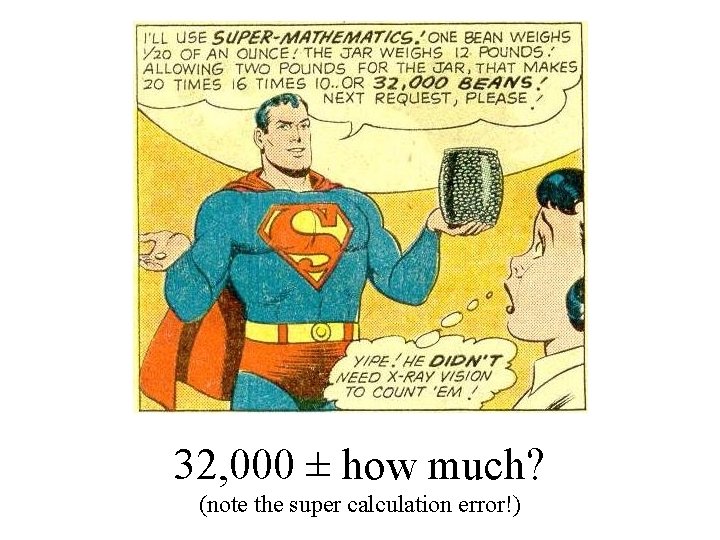
32, 000 ± how much? (note the super calculation error!)

Introduction to errors in data

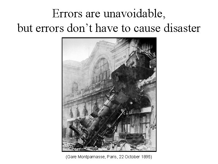
Errors are unavoidable, but errors don’t have to cause disaster (Gare Montparnasse, Paris, 22 October 1895)

Errors in data • Why do we have measurement errors?

Errors in data • Why do we have measurement errors? – – – Instrument errors, glitches, bugs Instrument calibration errors Imperfect instrument design, less-than-ideal application Instrument resolution “Problem of definition”: what are we trying to measure, anyway? • Errors are unavoidable and inevitable, but they can always be reduced • Errors are not necessarily bad, but not knowing what they are, or having an unrealistic view of what they are, is bad

Contemporary political perspective “There are knowns. These are things we know that we know. There are known unknowns. That is to say, there are things that we know we don't know. But there also unknowns. There are things we don't know. ” Donald Rumsfeld (February 12, 2002)

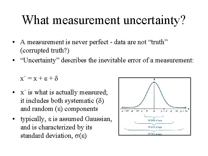
What measurement uncertainty? • A measurement is never perfect - data are not “truth” (corrupted truth? ) • “Uncertainty” describes the inevitable error of a measurement: x´ = x + + • x´ is what is actually measured; it includes both systematic ( ) and random ( ) components • typically, is assumed Gaussian, and is characterized by its standard deviation, ( )

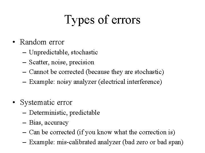
Types of errors • Random error – – Unpredictable, stochastic Scatter, noise, precision Cannot be corrected (because they are stochastic) Example: noisy analyzer (electrical interference) • Systematic error – – Deterministic, predictable Bias, accuracy Can be corrected (if you know what the correction is) Example: mis-calibrated analyzer (bad zero or bad span)

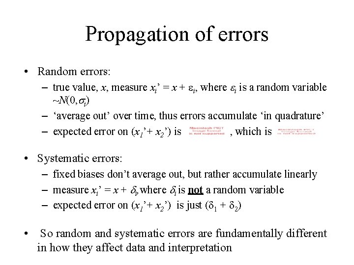
Propagation of errors • Random errors: – true value, x, measure xi’ = x + i, where ei is a random variable ~N(0, si) – ‘average out’ over time, thus errors accumulate ‘in quadrature’ – expected error on (x 1’+ x 2’) is , which is • Systematic errors: – fixed biases don’t average out, but rather accumulate linearly – measure xi’ = x + di, where di is not a random variable – expected error on (x 1’+ x 2’) is just ( 1 + 2) • So random and systematic errors are fundamentally different in how they affect data and interpretation

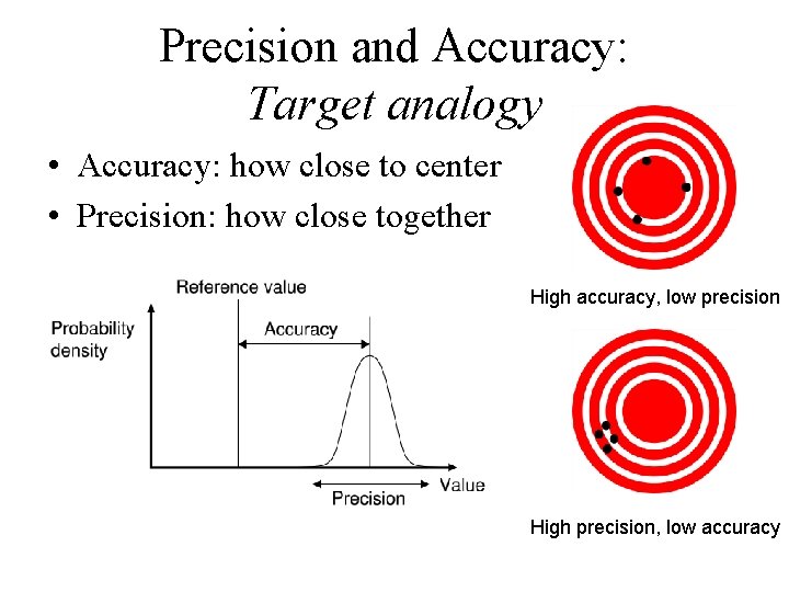
Precision and Accuracy: Target analogy • Accuracy: how close to center • Precision: how close together High accuracy, low precision High precision, low accuracy

Evaluating Errors • Random errors and precision – Make repeated measurements of the same thing – What is the scatter in those measurements? • Systematic errors and accuracy – Measure a reference standard – What is the bias? – Not always possible to quantify some systematic errors (know they’re there, but don’t have a standard we can measure)

What can we do about errors? • (Honestly) quantify sources of error – Random – Systematic • Minimize/eliminate them – Identify ways to reduce specific sources of error • Examples: more frequent calibration, better QC procedures, reduce instrument noise – Correct for biases where possible • Evaluate reductions in error

Why do we care about quantifying errors?

Why do we care about quantifying errors? • • • How much confidence do we have in the data? How certain are we about a particular measurement? How close to the “true” value are we? Are our data biased? In which direction? Errors influence our interpretation of data Errors reduce the usefulness of the information in our data • Errors in data propagate to subsequent analyses

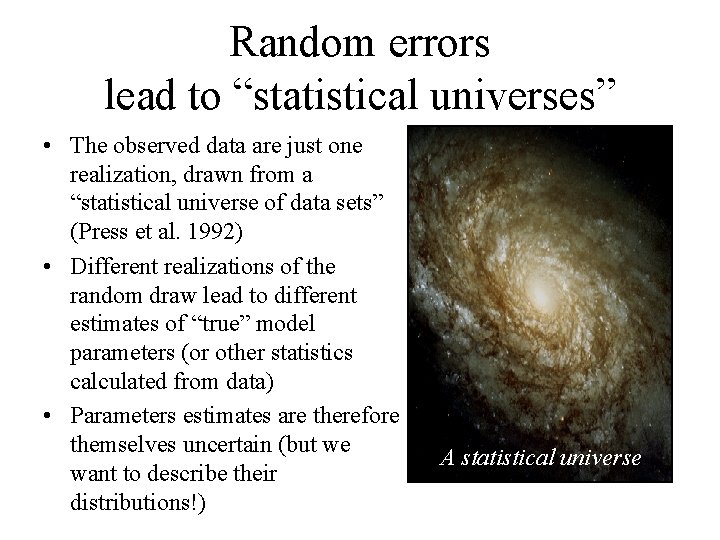
Random errors lead to “statistical universes” • The observed data are just one realization, drawn from a “statistical universe of data sets” (Press et al. 1992) • Different realizations of the random draw lead to different estimates of “true” model parameters (or other statistics calculated from data) • Parameters estimates are therefore themselves uncertain (but we want to describe their distributions!) A statistical universe

Monte Carlo Example • Two options for propagating errors – Complicated mathematics, based on theory and first principles – “Monte Carlo” simulations 1. Characterize uncertainty 2. Generate synthetic data (model + uncertainty) i. e. new realization from “statistical universe” 3. Estimate statistics or parameters, P, of interest 4. Repeat (2 & 3) many times 5. Posterior evaluation of distribution of P

Viva Las Vegas! “Offered the choice between mastery of a five-foot shelf of analytical statistics books and middling ability at performing statistical Monte Carlo simulations, we would surely choose to have the latter skill. ” William H. Press, Numerical Recipes in Fortran 77 Why you should learn a programming language (even fossil languages like BASIC): It’s really easy and fast to do MC simulations. In spreadsheet programs, it is extremely tedious (and slow), especially with large data sets (like you have with eddy flux data!).

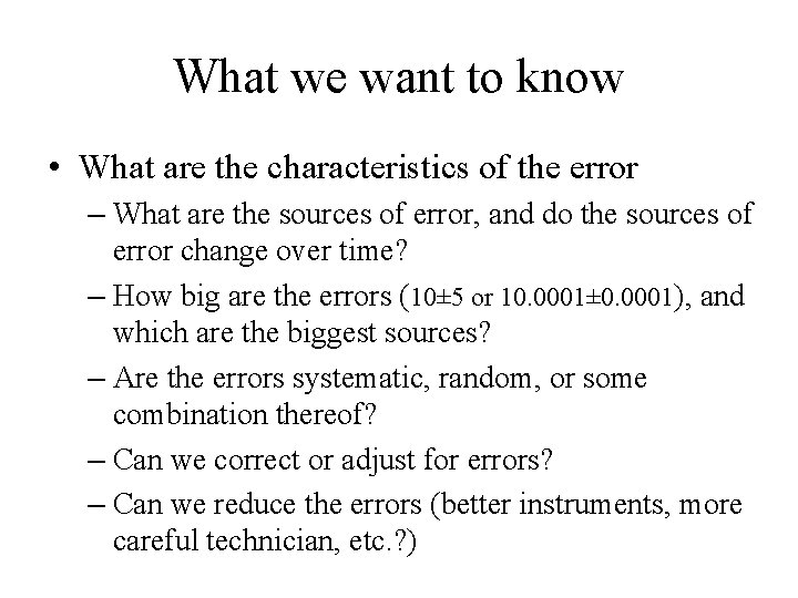
What we want to know • What are the characteristics of the error – What are the sources of error, and do the sources of error change over time? – How big are the errors (10± 5 or 10. 0001± 0. 0001), and which are the biggest sources? – Are the errors systematic, random, or some combination thereof? – Can we correct or adjust for errors? – Can we reduce the errors (better instruments, more careful technician, etc. ? )

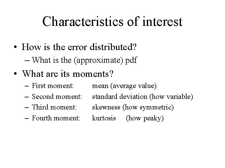
Characteristics of interest • How is the error distributed? – What is the (approximate) pdf • What are its moments? – – First moment: Second moment: Third moment: Fourth moment: mean (average value) standard deviation (how variable) skewness (how symmetric) kurtosis (how peaky)

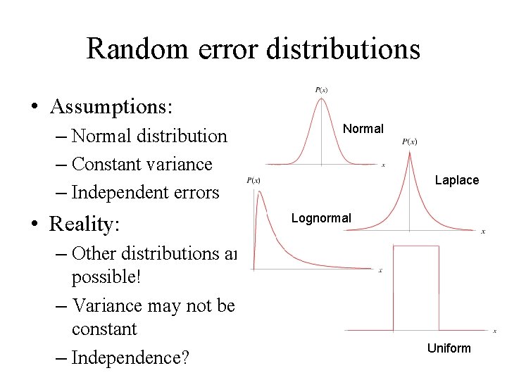
Random error distributions • Assumptions: – Normal distribution – Constant variance – Independent errors • Reality: – Other distributions are possible! – Variance may not be constant – Independence? Normal Laplace Lognormal Uniform

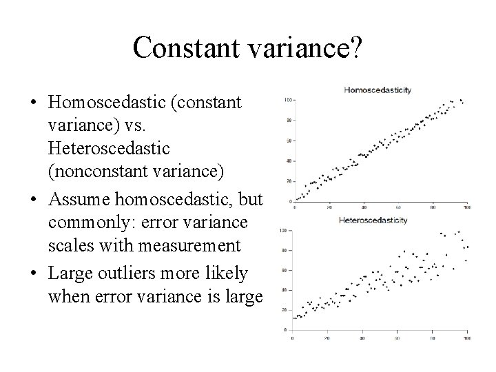
Constant variance? • Homoscedastic (constant variance) vs. Heteroscedastic (nonconstant variance) • Assume homoscedastic, but commonly: error variance scales with measurement • Large outliers more likely when error variance is large

Independence • Measurement error in period (t) are uncorrelated with errors in period (t-1) • Independent – coin toss (white noise) • Negative autocorrelation – growth rate estimated from size measurements • Positive autocorrelation – weekly biomass estimates confounded by seasonal variation in other factors (e. g. summer drought and shrinking xylem) • Difficult to detect or test for independence without a very good underlying model (with poor model, apparent autocorrelation may be due to model structure and not error structure!)

Take-home messages • For modelling, – More noise in data = more uncertainty in estimated model parameters – Systematic error in data = biased estimates of model parameters • Monte Carlo simulations as an easy way to evaluate impact of errors

Errors in flux measurements

Why characterize flux measurement uncertainty? • Uncertainty information needed to compare measurements, measurements and models, and to propagate errors (scaling up in space and time) • Uncertainty information needed to set policy & for risk analysis (what are confidence intervals on estimated C sink strength? ) • Uncertainty information needed for all aspects of data-model fusion (correct specification of cost function, forward prediction of states, etc. ) • Small uncertainties are not necessarily good; large uncertainties are not necessarily bad: biased prediction is ok if ‘truth’ is within confidence limits; if truth is outside of confidence limits, uncertainties are under-estimated

Challenge of flux data • Complex – Multiple processes (but only measure NEE) – Diurnal, synoptic, seasonal, annual scales of variation – Gaps in data (QC criteria, instrument malfunction, unsuitable weather, etc. ) • Multiple sources of error and uncertainty (known unknowns as well as unknowns!) • Random errors are large but tolerable • Systematic errors are evil, and the corrections for them are largely uncertain (sometimes even in sign) • Many sources of systematic error (sometimes in different directions)

Systematic errors Random errors

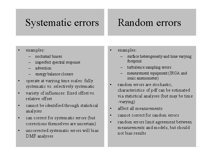
Systematic errors • examples: – – • • • Random errors • – nocturnal biases imperfect spectral response advection energy balance closure operate at varying time scales: fully systematic vs. selectively systematic variety of influences: fixed offset vs. relative offset cannot be identified through statistical analyses can correct for systematic errors (but corrections themselves are uncertain) uncorrected systematic errors will bias DMF analyses examples: – – • • surface heterogeneity and time varying footprint turbulence sampling errors measurement equipment (IRGA and sonic anemometer) random errors are stochastic; characteristics of pdf can be estimated via statistical analyses (but may be time -varying) affect all measurements cannot correct for random errors limit agreement between measurements and models, but should not bias results

How to estimate distributions of random flux errors

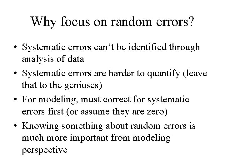
Why focus on random errors? • Systematic errors can’t be identified through analysis of data • Systematic errors are harder to quantify (leave that to the geniuses) • For modeling, must correct for systematic errors first (or assume they are zero) • Knowing something about random errors is much more important from modeling perspective

Two methods

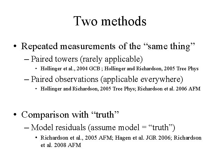
Two methods • Repeated measurements of the “same thing” – Paired towers (rarely applicable) • Hollinger et al. , 2004 GCB ; Hollinger and Richardson, 2005 Tree Phys – Paired observations (applicable everywhere) • Hollinger and Richardson, 2005 Tree Phys; Richardson et al. 2006 AFM • Comparison with “truth” – Model residuals (assume model = “truth”) • Richardson et al. , 2005 AFM; Hagen et al. JGR 2006; Richardson et al. 2008 AFM

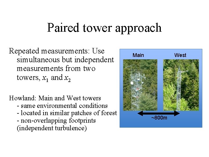
Paired tower approach Repeated measurements: Use simultaneous but independent measurements from two towers, x 1 and x 2 Howland: Main and West towers - same environmental conditions - located in similar patches of forest - non-overlapping footprints (independent turbulence) Main West ~800 m

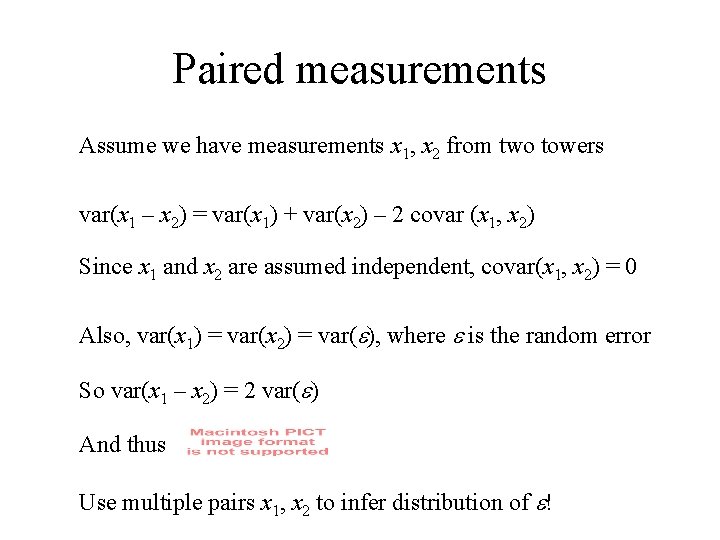
Paired measurements Assume we have measurements x 1, x 2 from two towers var(x 1 – x 2) = var(x 1) + var(x 2) – 2 covar (x 1, x 2) Since x 1 and x 2 are assumed independent, covar(x 1, x 2) = 0 Also, var(x 1) = var(x 2) = var(e), where e is the random error So var(x 1 – x 2) = 2 var(e) And thus Use multiple pairs x 1, x 2 to infer distribution of e!

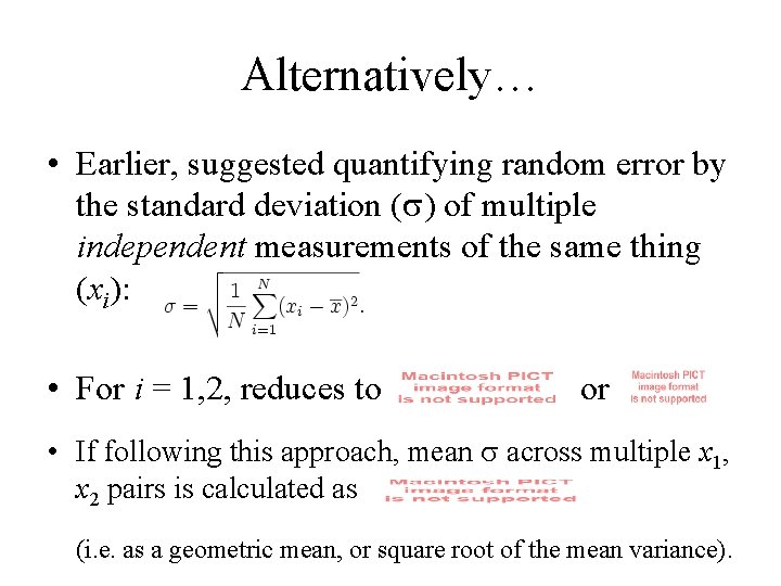
Alternatively… • Earlier, suggested quantifying random error by the standard deviation ( ) of multiple independent measurements of the same thing (xi): • For i = 1, 2, reduces to or • If following this approach, mean across multiple x 1, x 2 pairs is calculated as (i. e. as a geometric mean, or square root of the mean variance).

Another paired approach… • Two tower approach can only rarely be used • Alternative: substitute time for space – Use x 1, x 2 measured 24 h apart under similar environmental conditions • PPFD, VPD, Air/Soil temperature, Wind speed – Tradeoff: tight filtering criteria = not many paired measurements, poor estimates of statistics; loose filtering = other factors confound uncertainty estimate

Model residuals • Common in many fields (less so in “flux world”) to conduct posterior analyses of residuals to investigate pdf of errors, homoscedasticity, etc. • Disadvantage: – Model must be ‘good’ or uncertainty estimates confounded by model error • Advantages: – can evaluate asymmetry in error distribution (not possible with paired approach) – many data points with which to estimate statistics

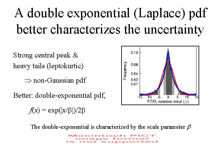
A double exponential (Laplace) pdf better characterizes the uncertainty Strong central peak & heavy tails (leptokurtic) Þ non-Gaussian pdf Better: double-exponential pdf, f(x) = exp(|x/ |)/2 The double-exponential is characterized by the scale parameter b

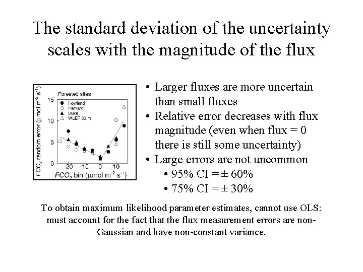
The standard deviation of the uncertainty scales with the magnitude of the flux • Larger fluxes are more uncertain than small fluxes • Relative error decreases with flux magnitude (even when flux = 0 there is still some uncertainty) • Large errors are not uncommon • 95% CI = ± 60% • 75% CI = ± 30% To obtain maximum likelihood parameter estimates, cannot use OLS: must account for the fact that the flux measurement errors are non. Gaussian and have non-constant variance.

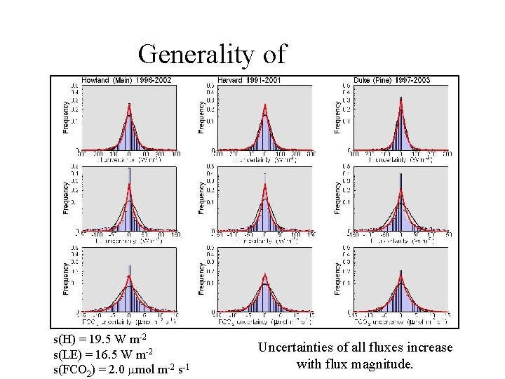
Generality of results • Scaling of uncertainty with flux magnitude has been validated using data from a range of forested Carbo. Europe sites: y-axis intercept (base uncertainty) varies among sites (factors: tower height, canopy roughness, average wind speed), but slope constant across sites (Richardson et al. , 2007) • Similar results (non-Gaussian, heteroscedastic) have been demonstrated for measurements of water and energy fluxes (H and LE) (Richardson et al. , 2006) • Results are in agreement with predictions of Mann and Lenschow (1994) error model based on turbulence statistics (Hollinger & Richardson, 2005; Richardson et al. , 2006)

Generality of results s(H) = 19. 5 W m-2 s(LE) = 16. 5 W m-2 s(FCO 2) = 2. 0 mmol m-2 s-1 Uncertainties of all fluxes increase with flux magnitude.

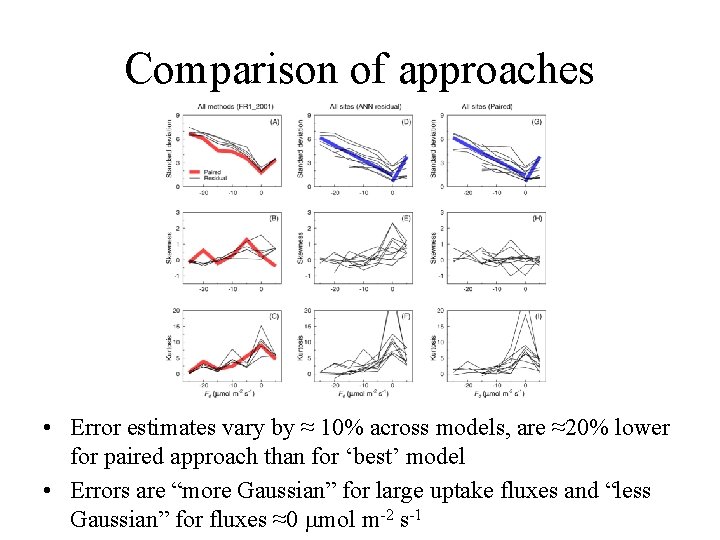
Comparison of approaches • Error estimates vary by ≈ 10% across models, are ≈20% lower for paired approach than for ‘best’ model • Errors are “more Gaussian” for large uptake fluxes and “less Gaussian” for fluxes ≈0 mmol m-2 s-1

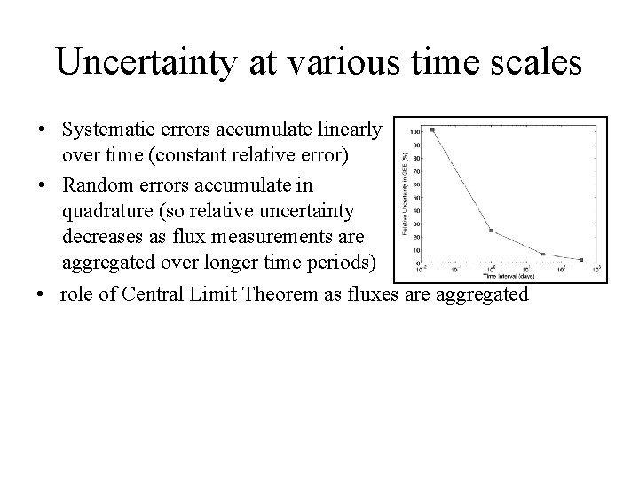
Uncertainty at various time scales • Systematic errors accumulate linearly over time (constant relative error) • Random errors accumulate in quadrature (so relative uncertainty decreases as flux measurements are aggregated over longer time periods) • role of Central Limit Theorem as fluxes are aggregated • Monte Carlo simulations suggest that uncertainty in annual NEE integrals uncertainty is ± 30 g C m-2 y-1 at 95% confidence (combination of random measurement error and associated uncertainty in gap filling) • Biases due to advection, etc. , are probably much larger than this but remain very hard to quantify

Implications for modeling

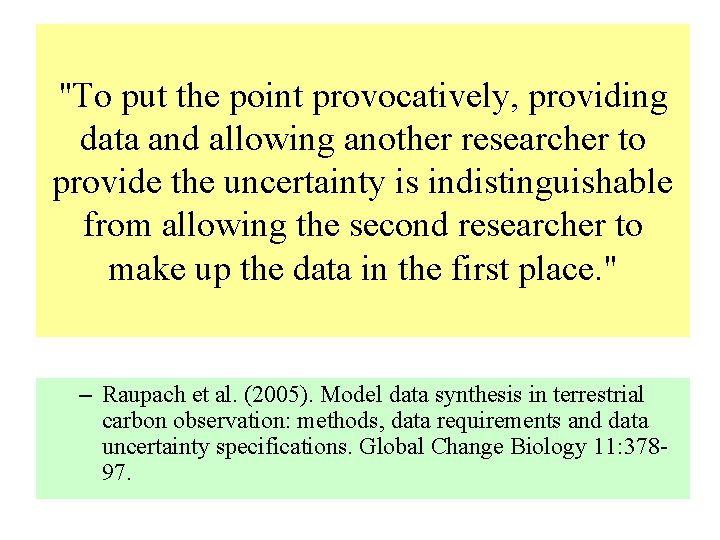
"To put the point provocatively, providing data and allowing another researcher to provide the uncertainty is indistinguishable from allowing the second researcher to make up the data in the first place. " – Raupach et al. (2005). Model data synthesis in terrestrial carbon observation: methods, data requirements and data uncertainty specifications. Global Change Biology 11: 37897.

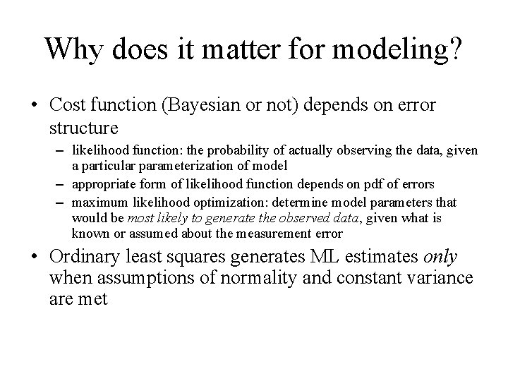
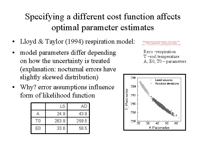
Why does it matter for modeling? • Cost function (Bayesian or not) depends on error structure – likelihood function: the probability of actually observing the data, given a particular parameterization of model – appropriate form of likelihood function depends on pdf of errors – maximum likelihood optimization: determine model parameters that would be most likely to generate the observed data, given what is known or assumed about the measurement error • Ordinary least squares generates ML estimates only when assumptions of normality and constant variance are met

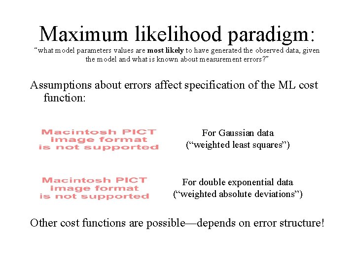
Maximum likelihood paradigm: “what model parameters values are most likely to have generated the observed data, given the model and what is known about measurement errors? ” Assumptions about errors affect specification of the ML cost function: For Gaussian data (“weighted least squares”) For double exponential data (“weighted absolute deviations”) Other cost functions are possible—depends on error structure!

Specifying a different cost function affects optimal parameter estimates • Lloyd & Taylor (1994) respiration model: • model parameters differ depending on how the uncertainty is treated (explanation: nocturnal errors have slightly skewed distribution) • Why? error assumptions influence form of likelihood function LS AD A 24. 9 43. 9 T 0 263. 9 259. 5 E 0 33. 6 58. 5 Reco –respiration T –soil temperature A, E 0, T 0 – parameters

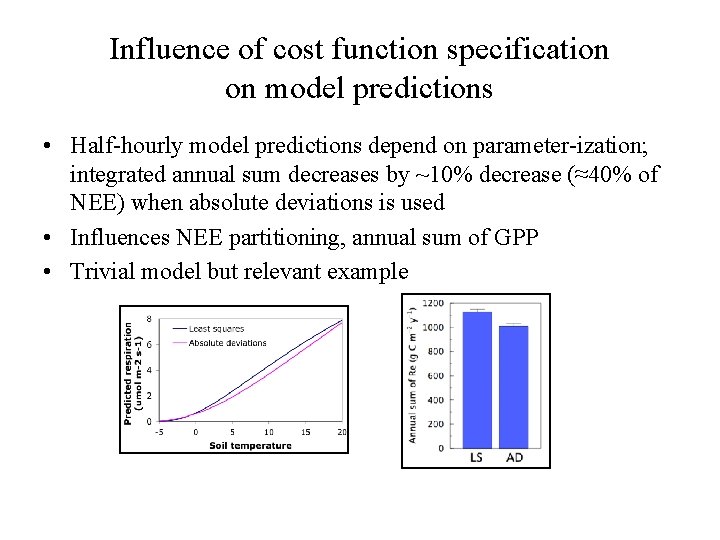
Influence of cost function specification on model predictions • Half-hourly model predictions depend on parameter-ization; integrated annual sum decreases by ~10% decrease (≈40% of NEE) when absolute deviations is used • Influences NEE partitioning, annual sum of GPP • Trivial model but relevant example

and also… • Random errors are stochastic noise – do not reflect “real” ecosystem activity – cannot be modeled because they are stochastic – ultimately limit agreement between models and data – make it difficult • to obtain precise parameter estimates (as shown by previous Monte Carlo example) • to select or distinguish among candidate models (more than one model gives acceptably good fit)

Summary • Two types of error, random and systematic • Random errors can be inferred from data • Flux measurement errors are non-Gaussian and have non-constant variance • These characteristics need to be taken into account when fitting models, when comparing models and data, and when estimating statistics from data (annual sums, physiological parameters, etc. )