The ChiSquare test Assistant prof Dr Mayasah A

The Chi-Square test Assistant prof. Dr. Mayasah A. Sadiq FICMS-FM 2 1

+ DATA QUALIT ATIVE CHI SQUARE TEST QUANTI TATIVE T-TEST

• The most obvious difference between the chi‑square tests and the other hypothesis tests we have considered (T test) is the nature of the data. • For chi‑square, the data are frequencies rather than numerical scores. 3

Chi-squared Tests • For testing significance of patterns in qualitative data. • Test statistic is based on counts that represent the number of items that fall in each category • Test statistics measures the agreement between actual counts(observed) and expected counts assuming the null hypothesis

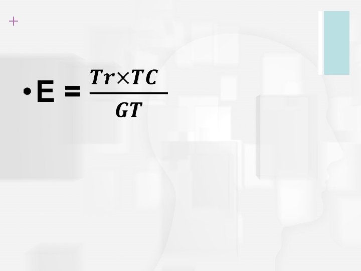
+ CHI SQUARE FORMULA:

Chi square distribution 6

Applications of Chi-square test: 1. Goodness-of-fit 2. The 2 x 2 chi-square test (contingency table, four fold table) 3. The a x b chi-square test (r x c chi-square test) 7

Steps of CHI hypothesis testing • 1. Data : counts or proportion. • 2. Assumption: random sample selected from a population. • 3. HO : no sign. Difference in proportion • no significant association. • HA: sign. Difference in proportion • significant association. 8

• • • 4. level of sign. df 1 st application=k-1(k is no. of groups) df 2 nd &3 rd application=(column-1)(row-1) IN 2 nd application(conengency table) Df=1, tab. Chi= 3. 841 always Graph is one side (only +ve) 9

• 5. apply appropriate test of significance 10

• • 6. Statistical decision & 7. Conclusion Calculated chi <tabulated chi P>0. 05 Accept HO, (may be true) If calculated chi> tabulated chi P<0. 05 Reject HO& accept HA. 11

The Chi-Square Test for Goodnessof-Fit • The chi-square test for goodness-of-fit uses frequency data from a sample to test hypotheses about the shape or proportions of a population. • The data, called observed frequencies, simply count how many individuals from the sample are in each category. 12

Example • • Eye colour in a sample of 40 Blue 12, brown 21, green 3, others 4 Eye colour in population Brown 80% Blue 10% Green 2% Others 8% Is there any difference between proportion of sample to that of population. use α 0. 05 13

Observed counts(frequency)

15

Expected counts(frequency) • • Expected blue 10/100*40=4 Expected brown=80/100*40=32 Expexcted green=2/100*40=0. 8 Expected others=8/100*40=3 16

1. Data • Represents the eye colour of 40 person in the following distribution • Brown=21 person, blue=12 person, green=3, others=4 17

2. Assumption • Sample is randomly selected from the population. 18

3. Hypothesis • Null hypothesis: there is no significant difference in proportion of eye colour of sample to that of the population. • Alternative hypothesis: there is significant difference in proportion of eye colour of sample to that of the population. 19

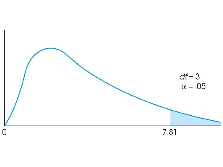
4. Level of significance; (α =0. 05); • 5% Chance factor effect area • 95% Influencing factor effect area • d. f. (degree of freedom)=K-1; (K=Number of subgroups) • =4 -1=3 • D. f. for 0. 5=7. 81 20

Accept Ho Influe ncing factor effect area 95% 5% Reject Ho Chance factor effect area 5% • 7. 81 21

5. Apply a proper test of significance 23

+ CHI SQUARE FORMULA:

+ 25

Observed counts(frequency)

27

Expected counts(frequency) • • Expected blue=10/100*40=4 Expected brown=80/100*40=32 Expexcted green=2/100*40=0. 8 Expected others=8/100*40=3 28

• =(12 -4)² (21 -32)² (3 -0. 8)² (4 -3)² • ------ +------ + ------- • 4 32 0. 8 3 • =(64/4) + (121/32)+(4. 8/0. 8)+(1/3) • =16+3. 78+6+0. 3= • Calculated chi =26. 08 29

Accept Ho Influe ncing factor effect area 95% 5% Reject Ho Chance factor effect area 5% • 7. 81 26. 08

6. Statistical decision • Calculated chi> tabulated chi • P<0. 5 31

7. Conclusion • We reject H 0 &accept HA: there is significant difference in proportion of eye colour of sample to that of the population. 32

Applications of Chi-square test: 1. Goodness-of-fit 2. The 2 x 2 chi-square test (contingency table, four fold table) 3. The a x b chi-square test (r x c chi-square test) 33

The Chi-Square Test for Independence • The second chi-square test, the chisquare test for independence, can be used and interpreted in two different ways: 1. Testing hypotheses about the relationship between two variables in a population, or(2× 2) 2. Testing hypotheses about differences between proportions for two or more populations. (a×b) 34

The Chi-Square Test for Independence (cont. ) • The data, called observed frequencies, simply show many individuals from the sample are in each cell of the matrix. • The null hypothesis for this test states that there is no relationship between the two variables; that is, the two variables are independent. 35

2 × 2 chi square (contingency table ) •

The Chi-Square Test for Independence (cont. ) The calculation of chi-square is the same for all chi-square tests: 37

+ CHI SQUARE FORMULA:

+ 2 nd application

+ Example • A total 1500 workers on 2 operators(A&B) • Were classified as deaf & non-deaf according to the following table. is there association between deafness & type of operator. let α 0. 05 40

Result Operator deaf not deaf. total A 100 900 1000 B 60 440 500 total 160 1340 1500

Result Operator deaf not deaf. total A 100 900 1000 B 60 440 500 total 160 1340 1500 Total number of items=1500 Total number of defective items=160

Result Operator def not def. total A 100 900 1000 B 60 440 500 total 160 1340 1500 Expected deaf from Operator A = 1000 * 160/1500 = 106. 7 (expected not deaf=1000 -106. 7=893. 3) Expected deaf from Operator B = 500 * 160/1500 = 53. 3

Result Operator def not def. total A 100 900 1000 B 60 440 500 total 160 1340 1500 A Expected not def. 893. 3 106. 7 B 53. 3 Operator total 446. 7 total

1. Data • Represent 1500 workers, 1000 on operator A 100 of them were deaf while 500 on operator B 60 of them were deaf 46

2. Assumption • Sample is randomly selected from the population. 47

3. Hypothesis • HO: there is no significant association between type of operator & deafness. • HA: there is significant association between type of operator & deafness. 48

4. Level of significance; (α = 0. 05); • 5% Chance factor effect area • 95% Influencing factor effect area • d. f. (degree of freedom)=(r-1)(c-1) =(2 -1)=1 • D. f. 1 for 0. 05=3. 841 49

Accept Ho Influe ncing factor effect area 95% 5% Reject Ho Chance factor effect area 5% • 3. 841

5. Apply a proper test of significance 51

+ 52

• • =(100 -106. 7)² ( 900 -893. 3)² (60 -53. 3)² --------------- + ------- 106. 7 893. 3 53. 3 +(440 -446. 7)² --------= 446. 7 =0. 42+0. 05+o. 84+0. 10 =1. 41 53

Accept Ho Influe ncing factor effect area 95% 5% Reject Ho Chance factor effect area 5% • 3. 841 1. 41

6. Statistical decision • Calculated chi< tabulated chi • P>0. 5 55

7. Conclusion • We accept H 0 • HO may be true • There is no significant association between type of operator & deafness. 56

Applications of Chi-square test: 1. Goodness-of-fit 2. The 2 x 2 chi-square test (contingency table, four fold table) 3. The a x b chi-square test (r x c chi-square test) 57

ₓ a b SA A NO D SD Gr 1 12 18 4 8 12 Gr 2 48 22 10 8 10 Gr 3 10 4 12 10 12

n

Degree of freedom The d. f depends on colunms number & rows number. or (r-1 ) (c-1) i. e. if 3 row , 4 colunms Df=(3 -1)(4 -1) df =6 If 3 rows, 3 colunms Df=(3 -1) Df=4

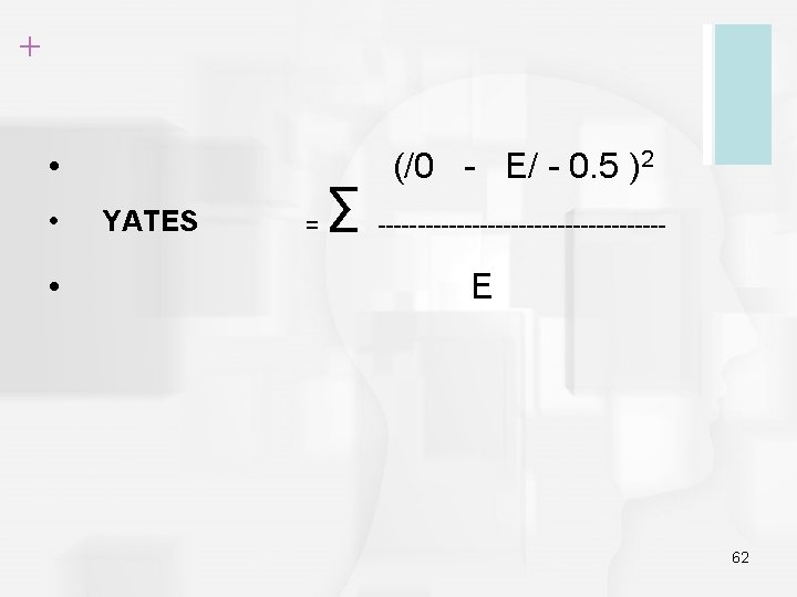
+ Yates Correction • When we apply 2 x 2 chi-square test and one of the expected cells was <5 • Or when we apply axb chi-square test and one of the expected cells was <2, • Or when the grand total is <40 • we have to apply Yates' correction formula; 61

+ Note • When 2 x 2 chi-square test have a zero cell (one of the four cells is zero) we can not apply chi-square test because we have what is called a complete dependence criteria. • But for axb chi-square test and one of the cells is zero when can not apply the test unless we do proper categorization to get rid of the zero cell. 63

+ 12 0 3 12 6 0 7 3 11 12 7 3 6 7 5 Or 5 5 13 64

+ 65